Vitamin B6, also called pyridoxine, is one of 8 B vitamins. Vitamin B6 is a water-soluble vitamin. There are three different natural forms of vitamin B6, namely pyridoxine, pyridoxamine, and pyridoxal, all of which are normally present in foods. For human metabolism the active derivative of the vitamin, pyridoxal 5-phosphate (PLP), is of major importance as the metabolically active coenzyme form.
Functions Make antibodies. Antibodies are needed to fight many diseases. Maintain normal nerve function Make hemoglobin. Hemoglobin carries oxygen in the red blood cells to the tissues. A vitamin B6 deficiency can cause a form of anemia. Break down proteins. The more protein you eat, the more vitamin B6 you need. Keep blood sugar (glucose) in normal ranges It’s significant to protein, fat and carbohydrate metabolism and the creation of red blood cells and neurotransmitters .Your body cannot produce vitamin B6, so you must obtain it from foods or supplements.
Over doses of vitamin B6 can cause: Difficulty coordinating movement Numbness Sensory changes Deficiency of this vitamin can cause: Difficulty coordinating movement Numbness Sensory changes Deficiency of this vitamin can cause: Confusion Depression Irritability Mouth and tongue sores (Vitamin B6 deficiency is not common in the United States.)
Deficiency
Vitamin B6 Deficiency of vitamin B6 leads to Neurological symptoms like depression, irritability, nervousness, mental confusion, convulsions and peripheral neuropathy glossitis, depression, hallucinations, muscle pains.
SUMMARY
Vitamin B6 may prevent a decline in brain function by decreasing homocysteine levels that have been associated with Alzheimer’s disease and memory impairments. However, studies have not proven the effectiveness of B6 in improving brain health.
Vitamin B12 is also called as Cyanocobalamin. Methylcobalamin and 5 deoxyadenosylcobalamin are the forms of vitamin B12 that are active in human metabolism.
Functions
Vitamin B12 is required for proper red blood cell formation and DNA synthesis. Vitamin B12 is also needed for building proteins in the body and normal function of nervous tissue Rich Foods 1) Beef liver 3 oz: 18 mcg (over 100% DV) 2) Sardines 3 oz: 7.6 mcg (over 100% DV) 3) Beef (grass-fed) 3 oz: 1.5 mcg (25% DV) 4) Tuna 3 oz: 2.5 mcg (41% DV) 5) Raw cheese 1.5 oz: 1.5 mcg (25% DV) 6) Cottage cheese 1 cup: 1.4 mcg (23% DV) 7) Lamb 3 oz: 2.07 mcg (35% DV) 8) Raw Milk 1 cup: 1.1 mcg (18% DV) 9) Eggs 1 large: 0.44 mcg (7% DV) 10) Salmon 3 oz: 1.1 mcg (18% DV)etc..
Overdose
Numbness, improper heart functioning, giddiness and regular headaches. The most serious side effect linked to overtime abuse of this vitamin, is increasing the risk of getting cancer.If you are undergoing pernicious anemia, an overdose of this vitamin can lead to leukemia.
If you are consuming a diet that has a high concentration of cholesterol along with different animal proteins, you stand a very high chance of getting cancer of the esophagus and stomach.
Deficiency
B12 Deficiency of vitamin B12 leads to strange sensations, numbness or tingling in the hands, legs or feet, difficulty walking (staggering, balance problems), anemia, a swollen, inflamed tongue,yellowed skin (jaundice).
The large molecules necessary for life that are built from smaller organic molecules are called biological macromolecules.
There are four major classes of biological macromolecules (carbohydrates, lipids, proteins, and nucleic acids), and each is an important component of the cell and performs a wide array of functions. Combined, these molecules make up the majority of a cell’s mass.
Biological macromolecules are organic, meaning that they contain carbon. In addition, they may contain hydrogen, oxygen, nitrogen, phosphorus, sulfur, and additional minor elements.
Carbon
It is often said that life is “carbon-based.” This means that carbon atoms, bonded to other carbon atoms or other elements, form the fundamental components of many, if not most, of the molecules found uniquely in living things.
Other elements play important roles in biological molecules, but carbon certainly qualifies as the “foundation” element for molecules in living things. It is the bonding properties of carbon atoms that are responsible for its important role.
Carbon Bonding
Carbon contains four electrons in its outer shell. Therefore, it can form four covalent bonds with other atoms or molecules. The simplest organic carbon molecule is methane (CH4), in which four hydrogen atoms bind to a carbon atom.
Figure :- Carbon can form four covalent bonds to create an organic molecule. The simplest carbon molecule is methane (CH4), depicted here.
However, structures that are more complex are made using carbon. Any of the hydrogen atoms can be replaced with another carbon atom covalently bonded to the first carbon atom. In this way, long and branching chains of carbon compounds can be made. The carbon atoms may bond with atoms of other elements, such as nitrogen, oxygen, and phosphorus.
The molecules may also form rings, which themselves can link with other rings . This diversity of molecular forms accounts for the diversity of functions of the biological macromolecules and is based to a large degree on the ability of carbon to form multiple bonds with itself and other atoms.
Figure :- These examples show three molecules (found in living organisms) that contain carbon atoms bonded in various ways to other carbon atoms and the atoms of other elements. (a) This molecule of stearic acid has a long chain of carbon atoms. (b) Glycine, a component of proteins, contains carbon, nitrogen, oxygen, and hydrogen atoms. (c) Glucose, a sugar, has a ring of carbon atoms and one oxygen atom.
Carbohydrates
Carbohydrates are macromolecules with which most consumers are somewhat familiar. To lose weight, some individuals adhere to “low-carb” diets. Athletes, in contrast, often “carb-load” before important competitions to ensure that they have sufficient energy to compete at a high level.
Carbohydrates are, in fact, an essential part of our diet; grains, fruits, and vegetables are all natural sources of carbohydrates. Carbohydrates provide energy to the body, particularly through glucose, a simple sugar. Carbohydrates also have other important functions in humans, animals, and plants.
Carbohydrates can be represented by the formula (CH2O)n, where n is the number of carbon atoms in the molecule. In other words, the ratio of carbon to hydrogen to oxygen is 1:2:1 in carbohydrate molecules. Carbohydrates are classified into three subtypes: monosaccharides, disaccharides, and polysaccharides.
Monosaccharides
Monosaccharides (mono- = “one”; sacchar- = “sweet”) are simple sugars, the most common of which is glucose. In monosaccharides, the number of carbon atoms usually ranges from three to six. Most monosaccharide names end with the suffix -ose. Depending on the number of carbon atoms in the sugar, they may be known as trioses (three carbon atoms), pentoses (five carbon atoms), and hexoses (six carbon atoms).
Monosaccharides may exist as a linear chain or as ring-shaped molecules; in aqueous solutions, they are usually found in the ring form.
The chemical formula for glucose is C6H12O6. In most living species, glucose is an important source of energy. During cellular respiration, energy is released from glucose, and that energy is used to help make adenosine triphosphate (ATP). Plants synthesize glucose using carbon dioxide and water by the process of photosynthesis, and the glucose, in turn, is used for the energy requirements of the plant. The excess synthesized glucose is often stored as starch that is broken down by other organisms that feed on plants.
Galactose (part of lactose, or milk sugar) and fructose (found in fruit) are other common monosaccharides. Although glucose, galactose, and fructose all have the same chemical formula (C6H12O6), they differ structurally and chemically (and are known as isomers) because of differing arrangements of atoms in the carbon chain.
Figure :- Glucose, galactose, and fructose are isomeric monosaccharides, meaning that they have the same chemical formula but slightly different structures.
Disaccharides (di- = “two”) form when two monosaccharides undergo a dehydration reaction (a reaction in which the removal of a water molecule occurs). During this process, the hydroxyl group (–OH) of one monosaccharide combines with a hydrogen atom of another monosaccharide, releasing a molecule of water (H2O) and forming a covalent bond between atoms in the two sugar molecules.
Common disaccharides include lactose, maltose, and sucrose. Lactose is a disaccharide consisting of the monomers glucose and galactose. It is found naturally in milk. Maltose, or malt sugar, is a disaccharide formed from a dehydration reaction between two glucose molecules. The most common disaccharide is sucrose, or table sugar, which is composed of the monomers glucose and fructose.
A long chain of monosaccharides linked by covalent bonds is known as a polysaccharide (poly- = “many”). The chain may be branched or unbranched, and it may contain different types of monosaccharides. Polysaccharides may be very large molecules. Starch, glycogen, cellulose, and chitin are examples of polysaccharides.
Starch is the stored form of sugars in plants and is made up of amylose and amylopectin (both polymers of glucose). Plants are able to synthesize glucose, and the excess glucose is stored as starch in different plant parts, including roots and seeds. The starch that is consumed by animals is broken down into smaller molecules, such as glucose. The cells can then absorb the glucose.
Glycogen is the storage form of glucose in humans and other vertebrates, and is made up of monomers of glucose. Glycogen is the animal equivalent of starch and is a highly branched molecule usually stored in liver and muscle cells. Whenever glucose levels decrease, glycogen is broken down to release glucose.
Cellulose is one of the most abundant natural biopolymers. The cell walls of plants are mostly made of cellulose, which provides structural support to the cell. Wood and paper are mostly cellulosic in nature. Cellulose is made up of glucose monomers that are linked by bonds between particular carbon atoms in the glucose molecule.
Every other glucose monomer in cellulose is flipped over and packed tightly as extended long chains. This gives cellulose its rigidity and high tensile strength—which is so important to plant cells. Cellulose passing through our digestive system is called dietary fiber. While the glucose-glucose bonds in cellulose cannot be broken down by human digestive enzymes, herbivores such as cows, buffalos, and horses are able to digest grass that is rich in cellulose and use it as a food source.
In these animals, certain species of bacteria reside in the rumen (part of the digestive system of herbivores) and secrete the enzyme cellulase. The appendix also contains bacteria that break down cellulose, giving it an important role in the digestive systems of ruminants. Cellulases can break down cellulose into glucose monomers that can be used as an energy source by the animal.
Carbohydrates serve other functions in different animals. Arthropods, such as insects, spiders, and crabs, have an outer skeleton, called the exoskeleton, which protects their internal body parts. This exoskeleton is made of the biological macromolecule chitin, which is a nitrogenous carbohydrate. It is made of repeating units of a modified sugar containing nitrogen.
Thus, through differences in molecular structure, carbohydrates are able to serve the very different functions of energy storage (starch and glycogen) and structural support and protection (cellulose and chitin).
Figure :- Although their structures and functions differ, all polysaccharide carbohydrates are made up of monosaccharides and have the chemical formula (CH2O)n.
Registered Dietitian: Obesity is a worldwide health concern, and many diseases, such as diabetes and heart disease, are becoming more prevalent because of obesity. This is one of the reasons why registered dietitians are increasingly sought after for advice.
Registered dietitians help plan food and nutrition programs for individuals in various settings. They often work with patients in health-care facilities, designing nutrition plans to prevent and treat diseases.
For example, dietitians may teach a patient with diabetes how to manage blood-sugar levels by eating the correct types and amounts of carbohydrates. Dietitians may also work in nursing homes, schools, and private practices.
To become a registered dietitian, one needs to earn at least a bachelor’s degree in dietetics, nutrition, food technology, or a related field. In addition, registered dietitians must complete a supervised internship program and pass a national exam.
Those who pursue careers in dietetics take courses in nutrition, chemistry, biochemistry, biology, microbiology, and human physiology. Dietitians must become experts in the chemistry and functions of food (proteins, carbohydrates, and fats).
The pH of a solution is a measure of its acidity or alkalinity. You have probably used litmus paper, paper that has been treated with a natural water-soluble dye so it can be used as a pH indicator, to test how much acid or base (alkalinity) exists in a solution. You might have even used some to make sure the water in an outdoor swimming pool is properly treated.
In both cases, this pH test measures the amount of hydrogen ions that exists in a given solution. High concentrations of hydrogen ions yield a low pH, whereas low levels of hydrogen ions result in a high pH. The overall concentration of hydrogen ions is inversely related to its pH and can be measured on the pH scale. Therefore, the more hydrogen ions present, the lower the pH; conversely, the fewer hydrogen ions, the higher the pH.
The pH scale ranges from 0 to 14. A change of one unit on the pH scale represents a change in the concentration of hydrogen ions by a factor of 10, a change in two units represents a change in the concentration of hydrogen ions by a factor of 100. Thus, small changes in pH represent large changes in the concentrations of hydrogen ions. Pure water is neutral.
It is neither acidic nor basic, and has a pH of 7.0. Anything below 7.0 (ranging from 0.0 to 6.9) is acidic, and anything above 7.0 (from 7.1 to 14.0) is alkaline. The blood in your veins is slightly alkaline (pH = 7.4). The environment in your stomach is highly acidic (pH = 1 to 2). Orange juice is mildly acidic (pH = approximately 3.5), whereas baking soda is basic (pH = 9.0).
The pH scale measures the amount of hydrogen ions (H+) in a substance. (credit: modification of work by Edward Stevens)
Acids are substances that provide hydrogen ions (H+) and lower pH, whereas bases provide hydroxide ions (OH–) and raise pH. The stronger the acid, the more readily it donates H+. For example, hydrochloric acid and lemon juice are very acidic and readily give up H+ when added to water.
Conversely, bases are those substances that readily donate OH–. The OH– ions combine with H+ to produce water, which raises a substance’s pH. Sodium hydroxide and many household cleaners are very alkaline and give up OH– rapidly when placed in water, thereby raising the pH.
Most cells in our bodies operate within a very narrow window of the pH scale, typically ranging only from 7.2 to 7.6. If the pH of the body is outside of this range, the respiratory system malfunctions, as do other organs in the body. Cells no longer function properly, and proteins will break down. Deviation outside of the pH range can induce coma or even cause death.
So how is it that we can ingest or inhale acidic or basic substances and not die? Buffers are the key. Buffers readily absorb excess H+ or OH–, keeping the pH of the body carefully maintained in the aforementioned narrow range.
Carbon dioxide is part of a prominent buffer system in the human body; it keeps the pH within the proper range. This buffer system involves carbonic acid (H2CO3) and bicarbonate (HCO3–) anion. If too much H+ enters the body, bicarbonate will combine with the H+ to create carbonic acid and limit the decrease in pH. Likewise, if too much OH– is introduced into the system, carbonic acid will rapidly dissociate into bicarbonate and H+ ions.
The H+ ions can combine with the OH– ions, limiting the increase in pH. While carbonic acid is an important product in this reaction, its presence is fleeting because the carbonic acid is released from the body as carbon dioxide gas each time we breathe. Without this buffer system, the pH in our bodies would fluctuate too much and we would fail to survive.
Section Summary
Water has many properties that are critical to maintaining life. It is polar, allowing for the formation of hydrogen bonds, which allow ions and other polar molecules to dissolve in water. Therefore, water is an excellent solvent. The hydrogen bonds between water molecules give water the ability to hold heat better than many other substances.
As the temperature rises, the hydrogen bonds between water continually break and reform, allowing for the overall temperature to remain stable, although increased energy is added to the system. Water’s cohesive forces allow for the property of surface tension. All of these unique properties of water are important in the chemistry of living organisms.
The pH of a solution is a measure of the concentration of hydrogen ions in the solution. A solution with a high number of hydrogen ions is acidic and has a low pH value. A solution with a high number of hydroxide ions is basic and has a high pH value. The pH scale ranges from 0 to 14, with a pH of 7 being neutral.
Buffers are solutions that moderate pH changes when an acid or base is added to the buffer system. Buffers are important in biological systems because of their ability to maintain constant pH conditions.
Reinforcement learning is a subfield of machine learning in which systems are trained by receiving virtual “rewards” or “punishments,” essentially learning by trial and error. Google’s DeepMind has used reinforcement learning to beat a human champion in the Go games. Reinforcement learning is also used in video games to improve the gaming experience by providing smarter bot.
One of the most famous algorithms are:
Q-learning
Deep Q network
State-Action-Reward-State-Action (SARSA)
Deep Deterministic Policy Gradient (DDPG)
Applications/ Examples of deep learning applications
AI in Finance: The financial technology sector has already started using AI to save time, reduce costs, and add value. Deep learning is changing the lending industry by using more robust credit scoring. Credit decision-makers can use AI for robust credit lending applications to achieve faster, more accurate risk assessment, using machine intelligence to factor in the character and capacity of applicants.
Underwrite is a Fintech company providing an AI solution for credit makers company. underwrite.ai uses AI to detect which applicant is more likely to pay back a loan. Their approach radically outperforms traditional methods.
AI in HR: Under Armour, a sportswear company revolutionizes hiring and modernizes the candidate experience with the help of AI. In fact, Under Armour Reduces hiring time for its retail stores by 35%. Under Armour faced a growing popularity interest back in 2012. They had, on average, 30000 resumes a month. Reading all of those applications and begin to start the screening and interview process was taking too long. The lengthy process to get people hired and on-boarded impacted Under Armour’s ability to have their retail stores fully staffed, ramped and ready to operate.
At that time, Under Armour had all of the ‘must have’ HR technology in place such as transactional solutions for sourcing, applying, tracking and onboarding but those tools weren’t useful enough. Under armour choose HireVue, an AI provider for HR solution, for both on-demand and live interviews. The results were bluffing; they managed to decrease by 35% the time to fill. In return, the hired higher quality staffs.
AI in Marketing: AI is a valuable tool for customer service management and personalization challenges. Improved speech recognition in call-center management and call routing as a result of the application of AI techniques allows a more seamless experience for customers.
For example, deep-learning analysis of audio allows systems to assess a customer’s emotional tone. If the customer is responding poorly to the AI chatbot, the system can be rerouted the conversation to real, human operators that take over the issue.
Apart from the three examples above, AI is widely used in other sectors/industries.
Why is Deep Learning Important?
Deep learning is a powerful tool to make prediction an actionable result. Deep learning excels in pattern discovery (unsupervised learning) and knowledge-based prediction. Big data is the fuel for deep learning. When both are combined, an organization can reap unprecedented results in term of productivity, sales, management, and innovation.
Deep learning can outperform traditional method. For instance, deep learning algorithms are 41% more accurate than machine learning algorithm in image classification, 27 % more accurate in facial recognition and 25% in voice recognition.
Limitations of deep learning
Data labeling
Most current AI models are trained through “supervised learning.” It means that humans must label and categorize the underlying data, which can be a sizable and error-prone chore. For example, companies developing self-driving-car technologies are hiring hundreds of people to manually annotate hours of video feeds from prototype vehicles to help train these systems.
Obtain huge training datasets
It has been shown that simple deep learning techniques like CNN can, in some cases, imitate the knowledge of experts in medicine and other fields. The current wave of machine learning, however, requires training data sets that are not only labeled but also sufficiently broad and universal.
Deep-learning methods required thousands of observation for models to become relatively good at classification tasks and, in some cases, millions for them to perform at the level of humans. Without surprise, deep learning is famous in giant tech companies; they are using big data to accumulate petabytes of data. It allows them to create an impressive and highly accurate deep learning model.
Explain a problem
Large and complex models can be hard to explain, in human terms. For instance, why a particular decision was obtained. It is one reason that acceptance of some AI tools are slow in application areas where interpretability is useful or indeed required.
Furthermore, as the application of AI expands, regulatory requirements could also drive the need for more explainable AI models.
Deep learning is the new state-of-the-art for artificial intelligence. Deep learning architecture is composed of an input layer, hidden layers, and an output layer. The word deep means there are more than two fully connected layers.
There is a vast amount of neural network, where each architecture is designed to perform a given task. For instance, CNN works very well with pictures, RNN provides impressive results with time series and text analysis.
Artificial Neural Network (ANN) it is an efficient computing system, whose central theme is borrowed from the analogy of biological neural networks. Neural networks are one type of model for machine learning. In the mid-1980s and early 1990s, much important architectural advancements were made in neural networks. In this chapter, you will learn more about Deep Learning, an approach of AI.
Deep learning emerged from a decade’s explosive computational growth as a serious contender in the field. Thus, deep learning is a particular kind of machine learning whose algorithms are inspired by the structure and function of human brain.
Machine Learning v/s Deep Learning
Deep learning is the most powerful machine learning technique these days. It is so powerful because they learn the best way to represent the problem while learning how to solve the problem. A comparison of Deep learning and Machine learning is given below −
Data Dependency
The first point of difference is based upon the performance of DL and ML when the scale of data increases. When the data is large, deep learning algorithms perform very well.
Machine Dependency
Deep learning algorithms need high-end machines to work perfectly. On the other hand, machine learning algorithms can work on low-end machines too.
Feature Extraction
Deep learning algorithms can extract high level features and try to learn from the same too. On the other hand, an expert is required to identify most of the features extracted by machine learning.
Time of Execution
Execution time depends upon the numerous parameters used in an algorithm. Deep learning has more parameters than machine learning algorithms. Hence, the execution time of DL algorithms, specially the training time, is much more than ML algorithms. But the testing time of DL algorithms is less than ML algorithms.
Approach to Problem Solving
Deep learning solves the problem end-to-end while machine learning uses the traditional way of solving the problem i.e. by breaking down it into parts.
Convolutional Neural Network (CNN)
Convolutional neural networks are the same as ordinary neural networks because they are also made up of neurons that have learnable weights and biases. Ordinary neural networks ignore the structure of input data and all the data is converted into 1-D array before feeding it into the network. This process suits the regular data, however if the data contains images, the process may be cumbersome.
CNN solves this problem easily. It takes the 2D structure of the images into account when they process them, which allows them to extract the properties specific to images. In this way, the main goal of CNNs is to go from the raw image data in the input layer to the correct class in the output layer. The only difference between an ordinary NNs and CNNs is in the treatment of input data and in the type of layers.
Architecture Overview of CNNs
Architecturally, the ordinary neural networks receive an input and transform it through a series of hidden layer. Every layer is connected to the other layer with the help of neurons. The main disadvantage of ordinary neural networks is that they do not scale well to full images.
The architecture of CNNs have neurons arranged in 3 dimensions called width, height and depth. Each neuron in the current layer is connected to a small patch of the output from the previous layer. It is similar to overlaying a 𝑵×𝑵filter on the input image. It uses M filters to be sure about getting all the details. These M filters are feature extractors which extract features like edges, corners, etc.
Layers used to construct CNNs
Following layers are used to construct CNNs −
· Input Layer − It takes the raw image data as it is.
· Convolutional Layer − This layer is the core building block of CNNs that does most of the computations. This layer computes the convolutions between the neurons and the various patches in the input.
· Rectified Linear Unit Layer − It applies an activation function to the output of the previous layer. It adds non-linearity to the network so that it can generalize well to any type of function.
· Pooling Layer − Pooling helps us to keep only the important parts as we progress in the network. Pooling layer operates independently on every depth slice of the input and resizes it spatially. It uses the MAX function.
· Fully Connected layer/Output layer − This layer computes the output scores in the last layer. The resulting output is of the size 𝟏×𝟏×𝑳 , where L is the number training dataset classes.
Installing Useful Python Packages
You can use Keras, which is an high level neural networks API, written in Python and capable of running on top of TensorFlow, CNTK or Theno. It is compatible with Python 2.7-3.6. You can learn more about it from https://keras.io/.
Use the following commands to install keras −
pip install keras
On conda environment, you can use the following command −
conda install –c conda-forge keras
Building Linear Regressor using ANN
In this section, you will learn how to build a linear regressor using artificial neural networks. You can use KerasRegressor to achieve this. In this example, we are using the Boston house price dataset with 13 numerical for properties in Boston. The Python code for the same is shown here −
Import all the required packages as shown −
import numpy
import pandas
from keras.models import Sequential
from keras.layers import Dense
from keras.wrappers.scikit_learn import KerasRegressor
from sklearn.model_selection import cross_val_score
from sklearn.model_selection import KFold
Now, load our dataset which is saved in local directory.
Now, fix the random seed for reproducibility as follows −
seed = 7
numpy.random.seed(seed)
The Keras wrapper object for use in scikit-learn as a regression estimator is called KerasRegressor. In this section, we shall evaluate this model with standardize data set.
The output of the code shown above would be the estimate of the model’s performance on the problem for unseen data. It will be the mean squared error, including the average and standard deviation across all 10 folds of the cross validation evaluation.
Image Classifier: An Application of Deep Learning
Convolutional Neural Networks (CNNs) solve an image classification problem, that is to which class the input image belongs to. You can use Keras deep learning library. Note that we are using the training and testing data set of images of cats and dogs from following link https://www.kaggle.com/c/dogs-vs-cats/data.
Import the important keras libraries and packages as shown −
The following package called sequential will initialize the neural networks as sequential network.
from keras.models import Sequential
The following package called Conv2D is used to perform the convolution operation, the first step of CNN.
from keras.layers import Conv2D
The following package called MaxPoling2D is used to perform the pooling operation, the second step of CNN.
from keras.layers import MaxPooling2D
The following package called Flatten is the process of converting all the resultant 2D arrays into a single long continuous linear vector.
from keras.layers import Flatten
The following package called Dense is used to perform the full connection of the neural network, the fourth step of CNN.
S_classifier.compile(optimizer = 'adam', loss = 'binary_crossentropy', metrics = ['accuracy'])
Here optimizer parameter is to choose the stochastic gradient descent algorithm, loss parameter is to choose the loss function and metrics parameter is to choose the performance metric.
Now, perform image augmentations and then fit the images to the neural networks −
A deep neural network provides state-of-the-art accuracy in many tasks, from object detection to speech recognition. They can learn automatically, without predefined knowledge explicitly coded by the programmers.
To grasp the idea of deep learning, imagine a family, with an infant and parents. The toddler points objects with his little finger and always says the word ‘cat.’ As its parents are concerned about his education, they keep telling him ‘Yes, that is a cat’ or ‘No, that is not a cat.’ The infant persists in pointing objects but becomes more accurate with ‘cats.’ The little kid, deep down, does not know why he can say it is a cat or not. He has just learned how to hierarchies complex features coming up with a cat by looking at the pet overall and continue to focus on details such as the tails or the nose before to make up his mind.
A neural network works quite the same. Each layer represents a deeper level of knowledge, i.e., the hierarchy of knowledge. A neural network with four layers will learn more complex feature than with that with two layers.
The learning occurs in two phases.
The first phase consists of applying a nonlinear transformation of the input and create a statistical model as output.
The second phase aims at improving the model with a mathematical method known as derivative.
The neural network repeats these two phases hundreds to thousands of time until it has reached a tolerable level of accuracy. The repeat of this two-phase is called an iteration.
To give an example, take a look at the motion below, the model is trying to learn how to dance. After 10 minutes of training, the model does not know how to dance, and it looks like a scribble.
After 48 hours of learning, the computer masters the art of dancing.
Classification of Neural Networks
Shallow neural network: The Shallow neural network has only one hidden layer between the input and output.
Deep neural network: Deep neural networks have more than one layer. For instance, Google LeNet model for image recognition counts 22 layers.
Nowadays, deep learning is used in many ways like a driverless car, mobile phone, Google Search Engine, Fraud detection, TV, and so on.
Types of Deep Learning Networks
Feed-forward neural networks
The simplest type of artificial neural network. With this type of architecture, information flows in only one direction, forward. It means, the information’s flows starts at the input layer, goes to the “hidden” layers, and end at the output layer. The network does not have a loop. Information stops at the output layers.
Recurrent neural networks (RNNs)
RNN is a multi-layered neural network that can store information in context nodes, allowing it to learn data sequences and output a number or another sequence. In simple words it an Artificial neural networks whose connections between neurons include loops. RNNs are well suited for processing sequences of inputs.
Example, if the task is to predict the next word in the sentence “Do you want a…………?
The RNN neurons will receive a signal that point to the start of the sentence.
The network receives the word “Do” as an input and produces a vector of the number. This vector is fed back to the neuron to provide a memory to the network. This stage helps the network to remember it received “Do” and it received it in the first position.
The network will similarly proceed to the next words. It takes the word “you” and “want.” The state of the neurons is updated upon receiving each word.
The final stage occurs after receiving the word “a.” The neural network will provide a probability for each English word that can be used to complete the sentence. A well-trained RNN probably assigns a high probability to “café,” “drink,” “burger,” etc.
Common uses of RNN
Help securities traders to generate analytic reports
Detect abnormalities in the contract of financial statement
Detect fraudulent credit-card transaction
Provide a caption for images
Power chatbots
The standard uses of RNN occur when the practitioners are working with time-series data or sequences (e.g., audio recordings or text).
“Composing Jazz Music with Deep Learning”
Deep Learning is on the rise, extending its application in every field, ranging from computer vision to natural language processing, healthcare, speech recognition, generating art, addition of sound to silent movies, machine translation, advertising, self-driving cars, etc. In this blog, we will extend the power of deep learning to the domain of music production. We will talk about how we can use deep learning to generate new musical beats.
The current technological advancements have transformed the way we produce music, listen, and work with music. With the advent of deep learning, it has now become possible to generate music without the need for working with instruments artists may not have had access to or the skills to use previously. This offers artists more creative freedom and ability to explore different domains of music.
Recurrent Neural Networks
Since music is a sequence of notes and chords, it doesn’t have a fixed dimensionality. Traditional deep neural network techniques cannot be applied to generate music as they assume the inputs and targets/outputs to have fixed dimensionality and outputs to be independent of each other. It is therefore clear that a domain-independent method that learns to map sequences to sequences would be useful.
Recurrent neural networks (RNNs) are a class of artificial neural networks that make use of sequential information present in the data.
A recurrent neural network has looped, or recurrent, connections which allow the network to hold information across inputs. These connections can be thought of as memory cells. In other words, RNNs can make use of information learned in the previous time step. As seen in Fig. 1, the output of the previous hidden/activation layer is fed into the next hidden layer. Such an architecture is efficient in learning sequence-based data.
In this blog, we will be using the Long Short-Term Memory (LSTM) architecture. LSTM is a type of recurrent neural network (proposed by Hochreiter and Schmidhuber, 1997) that can remember a piece of information and keep it saved for many timesteps.
Dataset
Our dataset includes piano tunes stored in the MIDI format. MIDI (Musical Instrument Digital Interface) is a protocol which allows electronic instruments and other digital musical tools to communicate with each other. Since a MIDI file only represents player information, i.e., a series of messages like ‘note on’, ‘note off, it is more compact, easy to modify, and can be adapted to any instrument.
Before we move forward, let us understand some music related terminologies:
· Note: A note is either a single sound or its representation in notation. Each note consist of pitch, octave, and an offset.
· Pitch: Pitch refers to the frequency of the sound.
· Octave: An octave is the interval between one musical pitch and another with half or double its frequency.
· Offset: Refers to the location of the note.
· Chord: Playing multiple notes at the same time constitutes a chord.
Machine Learning vs Deep Learning: What’s the Difference?
AI has three different levels:
Narrow AI: A artificial intelligence is said to be narrow when the machine can perform a specific task better than a human. The current research of AI is here now
General AI: An artificial intelligence reaches the general state when it can perform any intellectual task with the same accuracy level as a human would
Active AI: An AI is active when it can beat humans in many tasks
What is ML?
Machine learning is the best tool so far to analyze, understand and identify a pattern in the data. One of the main ideas behind machine learning is that the computer can be trained to automate tasks that would be exhaustive or impossible for a human being. The clear breach from the traditional analysis is that machine learning can take decisions with minimal human intervention.
Machine learning uses data to feed an algorithm that can understand the relationship between the input and the output. When the machine finished learning, it can predict the value or the class of new data point.
What is Deep Learning?
Deep learning is a computer software that mimics the network of neurons in a brain. It is a subset of machine learning and is called deep learning because it makes use of deep neural networks. The machine uses different layers to learn from the data. The depth of the model is represented by the number of layers in the model. Deep learning is the new state of the art in term of AI. In deep learning, the learning phase is done through a neural network. A neural network is an architecture where the layers are stacked on top of each other
Machine Learning Process
Imagine you are meant to build a program that recognizes objects. To train the model, you will use a classifier. A classifier uses the features of an object to try identifying the class it belongs to.
In the example, the classifier will be trained to detect if the image is a:
Bicycle
Boat
Car
Plane
The four objects above are the class the classifier has to recognize. To construct a classifier, you need to have some data as input and assigns a label to it. The algorithm will take these data, find a pattern and then classify it in the corresponding class.
This task is called supervised learning. In supervised learning, the training data you feed to the algorithm includes a label.
Training an algorithm requires to follow a few standard steps:
Collect the data
Train the classifier
Make predictions
The first step is necessary, choosing the right data will make the algorithm success or a failure. The data you choose to train the model is called a feature. In the object example, the features are the pixels of the images.
Each image is a row in the data while each pixel is a column. If your image is a 28×28 size, the dataset contains 784 columns (28×28). In the picture below, each picture has been transformed into a feature vector. The label tells the computer what object is in the image.
The objective is to use these training data to classify the type of object. The first step consists of creating the feature columns. Then, the second step involves choosing an algorithm to train the model. When the training is done, the model will predict what picture corresponds to what object.
After that, it is easy to use the model to predict new images. For each new image feeds into the model, the machine will predict the class it belongs to. For example, an entirely new image without a label is going through the model. For a human being, it is trivial to visualize the image as a car. The machine uses its previous knowledge to predict as well the image is a car.
Deep Learning Process
In deep learning, the learning phase is done through a neural network. A neural network is an architecture where the layers are stacked on top of each other.
Consider the same image example above. The training set would be fed to a neural network
Each input goes into a neuron and is multiplied by a weight. The result of the multiplication flows to the next layer and become the input. This process is repeated for each layer of the network. The final layer is named the output layer; it provides an actual value for the regression task and a probability of each class for the classification task. The neural network uses a mathematical algorithm to update the weights of all the neurons. The neural network is fully trained when the value of the weights gives an output close to the reality. For instance, a well-trained neural network can recognize the object on a picture with higher accuracy than the traditional neural net.
Automate Feature Extraction using DL
A dataset can contain a dozen to hundreds of features. The system will learn from the relevance of these features. However, not all features are meaningful for the algorithm. A crucial part of machine learning is to find a relevant set of features to make the system learns something.
One way to perform this part in machine learning is to use feature extraction. Feature extraction combines existing features to create a more relevant set of features. It can be done with PCA, T-SNE or any other dimensionality reduction algorithms.
For example, an image processing, the practitioner needs to extract the feature manually in the image like the eyes, the nose, lips and so on. Those extracted features are feed to the classification model.
Deep learning solves this issue, especially for a convolutional neural network. The first layer of a neural network will learn small details from the picture; the next layers will combine the previous knowledge to make more complex information. In the convolutional neural network, the feature extraction is done with the use of the filter. The network applies a filter to the picture to see if there is a match, i.e., the shape of the feature is identical to a part of the image. If there is a match, the network will use this filter. The process of feature extraction is therefore done automatically.
Difference between Machine Learning and Deep Learning
Machine Learning
Deep Learning
Data Dependencies
Excellent performances on a small/medium dataset
Excellent performance on a big dataset
Hardware dependencies
Work on a low-end machine.
Requires powerful machine, preferably with GPU: DL performs a significant amount of matrix multiplication
Feature engineering
Need to understand the features that represent the data
No need to understand the best feature that represents the data
Execution time
From few minutes to hours
Up to weeks. Neural Network needs to compute a significant number of weights
Interpretability
Some algorithms are easy to interpret (logistic, decision tree), some are almost impossible (SVM, XGBoost)
Difficult to impossible
When to use ML or DL?
In the table below, we summarize the difference between machine learning and deep learning.
Machine learning
Deep learning
Training dataset
Small
Large
Choose features
Yes
No
Number of algorithms
Many
Few
Training time
Short
Long
With machine learning, you need fewer data to train the algorithm than deep learning. Deep learning requires an extensive and diverse set of data to identify the underlying structure. Besides, machine learning provides a faster-trained model. Most advanced deep learning architecture can take days to a week to train.
The advantage of deep learning over machine learning is it is highly accurate. You do not need to understand what features are the best representation of the data; the neural network learned how to select critical features. In machine learning, you need to choose for yourself what features to include in the model.
Since the invention of computers or machines, their capability to perform various tasks has experienced an exponential growth. Humans have developed the power of computer systems in terms of their diverse working domains, their increasing speed, and reducing size with respect to time.
A branch of Computer Science named Artificial Intelligence pursues creating the computers or machines as intelligent as human beings.
Basic Concept of Artificial Intelligence (AI)
According to the father of Artificial Intelligence, John McCarthy, it is “The science and engineering of making intelligent machines, especially intelligent computer programs”.
Artificial Intelligence is a way of making a computer, a computer-controlled robot, or a software think intelligently, in the similar manner the intelligent humans think. AI is accomplished by studying how human brain thinks and how humans learn, decide, and work while trying to solve a problem, and then using the outcomes of this study as a basis of developing intelligent software and systems.
While exploiting the power of the computer systems, the curiosity of human, lead him to wonder, “Can a machine think and behave like humans do?”
Thus, the development of AI started with the intention of creating similar intelligence in machines that we find and regard high in humans.
The Necessity of Learning AI
As we know that AI pursues creating the machines as intelligent as human beings. There are numerous reasons for us to study AI. The reasons are as follows −
AI can learn through data
In our daily life, we deal with huge amount of data and human brain cannot keep track of so much data. That is why we need to automate the things. For doing automation, we need to study AI because it can learn from data and can do the repetitive tasks with accuracy and without tiredness.
AI can teach itself
It is very necessary that a system should teach itself because the data itself keeps changing and the knowledge which is derived from such data must be updated constantly. We can use AI to fulfill this purpose because an AI enabled system can teach itself.
AI can respond in real time
Artificial intelligence with the help of neural networks can analyze the data more deeply. Due to this capability, AI can think and respond to the situations which are based on the conditions in real time.
AI achieves accuracy
With the help of deep neural networks, AI can achieve tremendous accuracy. AI helps in the field of medicine to diagnose diseases such as cancer from the MRIs of patients.
AI can organize data to get most out of it
The data is an intellectual property for the systems which are using self-learning algorithms. We need AI to index and organize the data in a way that it always gives the best results.
Understanding Intelligence
With AI, smart systems can be built. We need to understand the concept of intelligence so that our brain can construct another intelligence system like itself.
What is Intelligence?
The ability of a system to calculate, reason, perceive relationships and analogies, learn from experience, store and retrieve information from memory, solve problems, comprehend complex ideas, use natural language fluently, classify, generalize, and adapt new situations.
Types of Intelligence
As described by Howard Gardner, an American developmental psychologist, Intelligence comes in multifold −
Sr.No
Intelligence & Description
Example
1
Linguistic intelligenceThe ability to speak, recognize, and use mechanisms of phonology (speech sounds), syntax (grammar), and semantics (meaning).
Narrators, Orators
2
Musical intelligenceThe ability to create, communicate with, and understand meanings made of sound, understanding of pitch, rhythm.
Musicians, Singers, Composers
3
Logical-mathematical intelligenceThe ability to use and understand relationships in the absence of action or objects. It is also the ability to understand complex and abstract ideas.
Mathematicians, Scientists
4
Spatial intelligenceThe ability to perceive visual or spatial information, change it, and re-create visual images without reference to the objects, construct 3D images, and to move and rotate them.
Map readers, Astronauts, Physicists
5
Bodily-Kinesthetic intelligenceThe ability to use complete or part of the body to solve problems or fashion products, control over fine and coarse motor skills, and manipulate the objects.
Players, Dancers
6
Intra-personal intelligenceThe ability to distinguish among one’s own feelings, intentions, and motivations.
Gautam Buddhha
7
Interpersonal intelligenceThe ability to recognize and make distinctions among other people’s feelings, beliefs, and intentions.
Mass Communicators, Interviewers
You can say a machine or a system is artificially intelligent when it is equipped with at least one or all intelligences in it.
What is Intelligence Composed Of?
The intelligence is intangible. It is composed of −
Reasoning
Learning
Problem Solving
Perception
Linguistic Intelligence
Let us go through all the components briefly −
Reasoning
It is the set of processes that enable us to provide basis for judgement, making decisions, and prediction. There are broadly two types −
Inductive Reasoning
Deductive Reasoning
It conducts specific observations to makes broad general statements.
It starts with a general statement and examines the possibilities to reach a specific, logical conclusion.
Even if all of the premises are true in a statement, inductive reasoning allows for the conclusion to be false.
If something is true of a class of things in general, it is also true for all members of that class.
Example − “Nita is a teacher. Nita is studious. Therefore, All teachers are studious.”
Example − “All women of age above 60 years are grandmothers. Shalini is 65 years. Therefore, Shalini is a grandmother.”
Learning − l
The ability of learning is possessed by humans, particular species of animals, and AI-enabled systems. Learning is categorized as follows −
Auditory Learning
It is learning by listening and hearing. For example, students listening to recorded audio lectures.
Episodic Learning
To learn by remembering sequences of events that one has witnessed or experienced. This is linear and orderly.
Motor Learning
It is learning by precise movement of muscles. For example, picking objects, writing, etc.
Observational Learning
To learn by watching and imitating others. For example, child tries to learn by mimicking her parent.
Perceptual Learning
It is learning to recognize stimuli that one has seen before. For example, identifying and classifying objects and situations.
Relational Learning
It involves learning to differentiate among various stimuli on the basis of relational properties, rather than absolute properties. For Example, Adding ‘little less’ salt at the time of cooking potatoes that came up salty last time, when cooked with adding say a tablespoon of salt.
· Spatial Learning − It is learning through visual stimuli such as images, colors, maps, etc. For example, A person can create roadmap in mind before actually following the road.
· Stimulus-Response Learning − It is learning to perform a particular behavior when a certain stimulus is present. For example, a dog raises its ear on hearing doorbell.
Problem Solving
It is the process in which one perceives and tries to arrive at a desired solution from a present situation by taking some path, which is blocked by known or unknown hurdles.
Problem solving also includes decision making, which is the process of selecting the best suitable alternative out of multiple alternatives to reach the desired goal.
Perception
It is the process of acquiring, interpreting, selecting, and organizing sensory information.
Perception presumes sensing. In humans, perception is aided by sensory organs. In the domain of AI, perception mechanism puts the data acquired by the sensors together in a meaningful manner.
Linguistic Intelligence
It is one’s ability to use, comprehend, speak, and write the verbal and written language. It is important in interpersonal communication.
What’s Involved in AI
Artificial intelligence is a vast area of study. This field of study helps in finding solutions to real world problems.
Let us now see the different fields of study within AI −
Machine Learning
It is one of the most popular fields of AI. The basic concept of this filed is to make the machine learning from data as the human beings can learn from his/her experience. It contains learning models on the basis of which the predictions can be made on unknown data.
Logic
It is another important field of study in which mathematical logic is used to execute the computer programs. It contains rules and facts to perform pattern matching, semantic analysis, etc.
Searching
This field of study is basically used in games like chess, tic-tac-toe. Search algorithms give the optimal solution after searching the whole search space.
Artificial neural networks
This is a network of efficient computing systems the central theme of which is borrowed from the analogy of biological neural networks. ANN can be used in robotics, speech recognition, speech processing, etc.
Genetic Algorithm
Genetic algorithms help in solving problems with the assistance of more than one program. The result would be based on selecting the fittest.
Knowledge Representation
It is the field of study with the help of which we can represent the facts in a way the machine that is understandable to the machine. The more efficiently knowledge is represented; the more system would be intelligent.
Application of AI
In this section, we will see the different fields supported by AI −
Gaming
AI plays crucial role in strategic games such as chess, poker, tic-tac-toe, etc., where machine can think of large number of possible positions based on heuristic knowledge.
Natural Language Processing
It is possible to interact with the computer that understands natural language spoken by humans.
Expert Systems
There are some applications which integrate machine, software, and special information to impart reasoning and advising. They provide explanation and advice to the users.
Vision Systems
These systems understand, interpret, and comprehend visual input on the computer. For example,
· A spying aeroplane takes photographs, which are used to figure out spatial information or map of the areas.
· Doctors use clinical expert system to diagnose the patient.
· Police use computer software that can recognize the face of criminal with the stored portrait made by forensic artist.
Speech Recognition
Some intelligent systems are capable of hearing and comprehending the language in terms of sentences and their meanings while a human talks to it. It can handle different accents, slang words, noise in the background, change in human’s noise due to cold, etc.
Handwriting Recognition
The handwriting recognition software reads the text written on paper by a pen or on screen by a stylus. It can recognize the shapes of the letters and convert it into editable text.
Intelligent Robots
Robots are able to perform the tasks given by a human. They have sensors to detect physical data from the real world such as light, heat, temperature, movement, sound, bump, and pressure. They have efficient processors, multiple sensors and huge memory, to exhibit intelligence. In addition, they are capable of learning from their mistakes and they can adapt to the new environment.
Cognitive Modeling: Simulating Human Thinking Procedure
Cognitive modeling is basically the field of study within computer science that deals with the study and simulating the thinking process of human beings. The main task of AI is to make machine think like human. The most important feature of human thinking process is problem solving. That is why more or less cognitive modeling tries to understand how humans can solve the problems. After that this model can be used for various AI applications such as machine learning, robotics, natural language processing, etc. Following is the diagram of different thinking levels of human brain −
Agent & Environment
In this section, we will focus on the agent and environment and how these help in Artificial Intelligence.
Agent
An agent is anything that can perceive its environment through sensors and acts upon that environment through effectors.
· A human agent has sensory organs such as eyes, ears, nose, tongue and skin parallel to the sensors, and other organs such as hands, legs, mouth, for effectors.
· A robotic agent replaces cameras and infrared range finders for the sensors, and various motors and actuators for effectors.
· A software agent has encoded bit strings as its programs and actions.
Environment
Some programs operate in an entirely artificial environment confined to keyboard input, database, computer file systems and character output on a screen.
In contrast, some software agents (software robots or softbots) exist in rich, unlimited softbots domains. The simulator has a very detailed, complex environment. The software agent needs to choose from a long array of actions in real time. A softbot is designed to scan the online preferences of the customer and shows interesting items to the customer works in the real as well as an artificial environment.
“AI with Python – Getting Started”
In this chapter, we will learn how to get started with Python. We will also understand how Python helps for Artificial Intelligence.
Why Python for AI
Artificial intelligence is considered to be the trending technology of the future. Already there are a number of applications made on it. Due to this, many companies and researchers are taking interest in it. But the main question that arises here is that in which programming language can these AI applications be developed? There are various programming languages like Lisp, Prolog, C++, Java and Python, which can be used for developing applications of AI. Among them, Python programming language gains a huge popularity and the reasons are as follows −
Simple syntax & less coding
Python involves very less coding and simple syntax among other programming languages which can be used for developing AI applications. Due to this feature, the testing can be easier and we can focus more on programming.
Inbuilt libraries for AI projects
A major advantage for using Python for AI is that it comes with inbuilt libraries. Python has libraries for almost all kinds of AI projects. For example, NumPy, SciPy, matplotlib, nltk, SimpleAI are some the important inbuilt libraries of Python.
· Open source − Python is an open source programming language. This makes it widely popular in the community.
· Can be used for broad range of programming − Python can be used for a broad range of programming tasks like small shell script to enterprise web applications. This is another reason Python is suitable for AI projects.
Features of Python
Python is a high-level, interpreted, interactive and object-oriented scripting language. Python is designed to be highly readable. It uses English keywords frequently where as other languages use punctuation, and it has fewer syntactical constructions than other languages. Python’s features include the following −
· Easy-to-learn − Python has few keywords, simple structure, and a clearly defined syntax. This allows the student to pick up the language quickly.
· Easy-to-read − Python code is more clearly defined and visible to the eyes.
· Easy-to-maintain − Python’s source code is fairly easy-to-maintain.
· A broad standard library − Python’s bulk of the library is very portable and cross-platform compatible on UNIX, Windows, and Macintosh.
· Interactive Mode − Python has support for an interactive mode which allows interactive testing and debugging of snippets of code.
· Portable − Python can run on a wide variety of hardware platforms and has the same interface on all platforms.
· Extendable − We can add low-level modules to the Python interpreter. These modules enable programmers to add to or customize their tools to be more efficient.
· Databases − Python provides interfaces to all major commercial databases.
· GUI Programming − Python supports GUI applications that can be created and ported to many system calls, libraries and windows systems, such as Windows MFC, Macintosh, and the X Window system of Unix.
· Scalable − Python provides a better structure and support for large programs than shell scripting.
Important features of Python
Let us now consider the following important features of Python −
· It supports functional and structured programming methods as well as OOP.
· It can be used as a scripting language or can be compiled to byte-code for building large applications.
· It provides very high-level dynamic data types and supports dynamic type checking.
· It supports automatic garbage collection.
· It can be easily integrated with C, C++, COM, ActiveX, CORBA, and Java.
Installing Python
Python distribution is available for a large number of platforms. You need to download only the binary code applicable for your platform and install Python.
If the binary code for your platform is not available, you need a C compiler to compile the source code manually. Compiling the source code offers more flexibility in terms of choice of features that you require in your installation.
Here is a quick overview of installing Python on various platforms −
Unix and Linux Installation
Follow these steps to install Python on Unix/Linux machine.
· Follow the link for the Windows installer python-XYZ.msi file where XYZ is the version you need to install.
· To use this installer python-XYZ.msi, the Windows system must support Microsoft Installer 2.0. Save the installer file to your local machine and then run it to find out if your machine supports MSI.
· Run the downloaded file. This brings up the Python install wizard, which is really easy to use. Just accept the default settings and wait until the install is finished.
Macintosh Installation
If you are on Mac OS X, it is recommended that you use Homebrew to install Python 3. It is a great package installer for Mac OS X and it is really easy to use. If you don’t have Homebrew, you can install it using the following command −
We can update the package manager with the command below −
$ brew update
Now run the following command to install Python3 on your system −
$ brew install python3
Setting up PATH
Programs and other executable files can be in many directories, so operating systems provide a search path that lists the directories that the OS searches for executables.
The path is stored in an environment variable, which is a named string maintained by the operating system. This variable contains information available to the command shell and other programs.
The path variable is named as PATH in Unix or Path in Windows (Unix is case-sensitive; Windows is not).
In Mac OS, the installer handles the path details. To invoke the Python interpreter from any particular directory, you must add the Python directory to your path.
Setting Path at Unix/Linux
To add the Python directory to the path for a particular session in Unix −
· In the csh shell
Type setenv PATH “$PATH:/usr/local/bin/python” and press Enter.
· In the bash shell (Linux)
Type export ATH = “$PATH:/usr/local/bin/python” and press Enter.
· In the sh or ksh shell
Type PATH = “$PATH:/usr/local/bin/python” and press Enter.
Note − /usr/local/bin/python is the path of the Python directory.
Setting Path at Windows
To add the Python directory to the path for a particular session in Windows −
· At the command prompt − type path %path%;C:\Python and press Enter.
Note − C:\Python is the path of the Python directory.
Running Python
Let us now see the different ways to run Python. The ways are described below −
Interactive Interpreter
We can start Python from Unix, DOS, or any other system that provides you a command-line interpreter or shell window.
· Enter python at the command line.
· Start coding right away in the interactive interpreter.
$python # Unix/Linux
or
python% # Unix/Linux
or
C:> python # Windows/DOS
Here is the list of all the available command line options −
S.No.
Option & Description
1
-dIt provides debug output.
2
-oIt generates optimized bytecode (resulting in .pyo files).
3
-SDo not run import site to look for Python paths on startup.
4
-vVerbose output (detailed trace on import statements).
5
-xDisables class-based built-in exceptions (just use strings); obsolete starting with version 1.6.
6
-c cmdRuns Python script sent in as cmd string.
7
FileRun Python script from given file.
Script from the Command-line
A Python script can be executed at the command line by invoking the interpreter on your application, as in the following −
$python script.py # Unix/Linux
or,
python% script.py # Unix/Linux
or,
C:> python script.py # Windows/DOS
Note − Be sure the file permission mode allows execution.
Integrated Development Environment
You can run Python from a Graphical User Interface (GUI) environment as well, if you have a GUI application on your system that supports Python.
· Unix − IDLE is the very first Unix IDE for Python.
· Windows − PythonWin is the first Windows interface for Python and is an IDE with a GUI.
· Macintosh − The Macintosh version of Python along with the IDLE IDE is available from the main website, downloadable as either MacBinary or BinHex’d files.
If you are not able to set up the environment properly, then you can take help from your system admin. Make sure the Python environment is properly set up and working perfectly fine.
We can also use another Python platform called Anaconda. It includes hundreds of popular data science packages and the conda package and virtual environment manager for Windows, Linux and MacOS. You can download it as per your operating system from the link https://www.anaconda.com/download/.
“AI with Python – Machine Learning”
Learning means the acquisition of knowledge or skills through study or experience. Based on this, we can define machine learning (ML) as follows −
It may be defined as the field of computer science, more specifically an application of artificial intelligence, which provides computer systems the ability to learn with data and improve from experience without being explicitly programmed.
Basically, the main focus of machine learning is to allow the computers learn automatically without human intervention. Now the question arises that how such learning can be started and done? It can be started with the observations of data. The data can be some examples, instruction or some direct experiences too. Then on the basis of this input, machine makes better decision by looking for some patterns in data.
Types of Machine Learning (ML)
Machine Learning Algorithms helps computer system learn without being explicitly programmed. These algorithms are categorized into supervised or unsupervised. Let us now see a few algorithms −
Supervised machine learning algorithms
This is the most commonly used machine learning algorithm. It is called supervised because the process of algorithm learning from the training dataset can be thought of as a teacher supervising the learning process. In this kind of ML algorithm, the possible outcomes are already known and training data is also labeled with correct answers. It can be understood as follows −
Suppose we have input variables x and an output variable y and we applied an algorithm to learn the mapping function from the input to output such as −
Y = f(x)
Now, the main goal is to approximate the mapping function so well that when we have new input data (x), we can predict the output variable (Y) for that data.
Mainly supervised leaning problems can be divided into the following two kinds of problems −
· Classification − A problem is called classification problem when we have the categorized output such as “black”, “teaching”, “non-teaching”, etc.
· Regression − A problem is called regression problem when we have the real value output such as “distance”, “kilogram”, etc.
Decision tree, random forest, knn, logistic regression are the examples of supervised machine learning algorithms.
Unsupervised machine learning algorithms
As the name suggests, these kinds of machine learning algorithms do not have any supervisor to provide any sort of guidance. That is why unsupervised machine learning algorithms are closely aligned with what some call true artificial intelligence. It can be understood as follows −
Suppose we have input variable x, then there will be no corresponding output variables as there is in supervised learning algorithms.
In simple words, we can say that in unsupervised learning there will be no correct answer and no teacher for the guidance. Algorithms help to discover interesting patterns in data.
Unsupervised learning problems can be divided into the following two kinds of problem −
· Clustering − In clustering problems, we need to discover the inherent groupings in the data. For example, grouping customers by their purchasing behavior.
· Association − A problem is called association problem because such kinds of problem require discovering the rules that describe large portions of our data. For example, finding the customers who buy both x and y.
K-means for clustering, Apriori algorithm for association are the examples of unsupervised machine learning algorithms.
Reinforcement machine learning algorithms
These kinds of machine learning algorithms are used very less. These algorithms train the systems to make specific decisions. Basically, the machine is exposed to an environment where it trains itself continually using the trial and error method. These algorithms learn from past experience and tries to capture the best possible knowledge to make accurate decisions. Markov Decision Process is an example of reinforcement machine learning algorithms.
Most Common Machine Learning Algorithms
In this section, we will learn about the most common machine learning algorithms. The algorithms are described below −
Linear Regression
It is one of the most well-known algorithms in statistics and machine learning.
Basic concept − Mainly linear regression is a linear model that assumes a linear relationship between the input variables say x and the single output variable say y. In other words, we can say that y can be calculated from a linear combination of the input variables x. The relationship between variables can be established by fitting a best line.
Types of Linear Regression
Linear regression is of the following two types −
· Simple linear regression − A linear regression algorithm is called simple linear regression if it is having only one independent variable.
· Multiple linear regression − A linear regression algorithm is called multiple linear regression if it is having more than one independent variable.
Linear regression is mainly used to estimate the real values based on continuous variable(s). For example, the total sale of a shop in a day, based on real values, can be estimated by linear regression.
Logistic Regression
It is a classification algorithm and also known as logit regression.
Mainly logistic regression is a classification algorithm that is used to estimate the discrete values like 0 or 1, true or false, yes or no based on a given set of independent variable. Basically, it predicts the probability hence its output lies in between 0 and 1.
Decision Tree
Decision tree is a supervised learning algorithm that is mostly used for classification problems.
Basically it is a classifier expressed as recursive partition based on the independent variables. Decision tree has nodes which form the rooted tree. Rooted tree is a directed tree with a node called “root”. Root does not have any incoming edges and all the other nodes have one incoming edge. These nodes are called leaves or decision nodes. For example, consider the following decision tree to see whether a person is fit or not.
Support Vector Machine (SVM)
It is used for both classification and regression problems. But mainly it is used for classification problems. The main concept of SVM is to plot each data item as a point in n-dimensional space with the value of each feature being the value of a particular coordinate. Here n would be the features we would have. Following is a simple graphical representation to understand the concept of SVM −
In the above diagram, we have two features hence we first need to plot these two variables in two dimensional space where each point has two co-ordinates, called support vectors. The line splits the data into two different classified groups. This line would be the classifier.
Naïve Bayes
It is also a classification technique. The logic behind this classification technique is to use Bayes theorem for building classifiers. The assumption is that the predictors are independent. In simple words, it assumes that the presence of a particular feature in a class is unrelated to the presence of any other feature. Below is the equation for Bayes theorem −
P(AB)=P(BA)P(A)P(B)P(AB)=P(BA)P(A)P(B)
The Naïve Bayes model is easy to build and particularly useful for large data sets.
K-Nearest Neighbors (KNN)
It is used for both classification and regression of the problems. It is widely used to solve classification problems. The main concept of this algorithm is that it used to store all the available cases and classifies new cases by majority votes of its k neighbors. The case being then assigned to the class which is the most common amongst its K-nearest neighbors, measured by a distance function. The distance function can be Euclidean, Minkowski and Hamming distance. Consider the following to use KNN −
· Computationally KNN are expensive than other algorithms used for classification problems.
· The normalization of variables needed otherwise higher range variables can bias it.
· In KNN, we need to work on pre-processing stage like noise removal.
K-Means Clustering
As the name suggests, it is used to solve the clustering problems. It is basically a type of unsupervised learning. The main logic of K-Means clustering algorithm is to classify the data set through a number of clusters. Follow these steps to form clusters by K-means −
· K-means picks k number of points for each cluster known as centroids.
· Now each data point forms a cluster with the closest centroids, i.e., k clusters.
· Now, it will find the centroids of each cluster based on the existing cluster members.
· We need to repeat these steps until convergence occurs.
Random Forest
It is a supervised classification algorithm. The advantage of random forest algorithm is that it can be used for both classification and regression kind of problems. Basically it is the collection of decision trees (i.e., forest) or you can say ensemble of the decision trees. The basic concept of random forest is that each tree gives a classification and the forest chooses the best classifications from them. Followings are the advantages of Random Forest algorithm −
· Random forest classifier can be used for both classification and regression tasks.
· They can handle the missing values.
· It won’t over fit the model even if we have more number of trees in the forest.
AI with Python – Data Preparation
We have already studied supervised as well as unsupervised machine learning algorithms. These algorithms require formatted data to start the training process. We must prepare or format data in a certain way so that it can be supplied as an input to ML algorithms.
This chapter focuses on data preparation for machine learning algorithms.
Preprocessing the Data
In our daily life, we deal with lots of data but this data is in raw form. To provide the data as the input of machine learning algorithms, we need to convert it into a meaningful data. That is where data preprocessing comes into picture. In other simple words, we can say that before providing the data to the machine learning algorithms we need to preprocess the data.
Data preprocessing steps
Follow these steps to preprocess the data in Python −
Step 1 − Importing the useful packages − If we are using Python then this would be the first step for converting the data into a certain format, i.e., preprocessing. It can be done as follows −
import numpy as np
sklearn import preprocessing
Here we have used the following two packages −
· NumPy − Basically NumPy is a general purpose array-processing package designed to efficiently manipulate large multi-dimensional arrays of arbitrary records without sacrificing too much speed for small multi-dimensional arrays.
· Sklearn.preprocessing − This package provides many common utility functions and transformer classes to change raw feature vectors into a representation that is more suitable for machine learning algorithms.
Step 2 − Defining sample data − After importing the packages, we need to define some sample data so that we can apply preprocessing techniques on that data. We will now define the following sample data −
Input_data = np.array([2.1, -1.9, 5.5],
[-1.5, 2.4, 3.5],
[0.5, -7.9, 5.6],
[5.9, 2.3, -5.8]])
Step3 − Applying preprocessing technique − In this step, we need to apply any of the preprocessing techniques.
The following section describes the data preprocessing techniques.
Techniques for Data Preprocessing
The techniques for data preprocessing are described below −
Binarization
This is the preprocessing technique which is used when we need to convert our numerical values into Boolean values. We can use an inbuilt method to binarize the input data say by using 0.5 as the threshold value in the following way −
Now, after running the above code we will get the following output, all the values above 0.5(threshold value) would be converted to 1 and all the values below 0.5 would be converted to 0.
Binarized data
[[ 1. 0. 1.]
[ 0. 1. 1.]
[ 0. 0. 1.]
[ 1. 1. 0.]]
Mean Removal
It is another very common preprocessing technique that is used in machine learning. Basically it is used to eliminate the mean from feature vector so that every feature is centered on zero. We can also remove the bias from the features in the feature vector. For applying mean removal preprocessing technique on the sample data, we can write the Python code shown below. The code will display the Mean and Standard deviation of the input data −
We will get the following output after running the above lines of code −
Mean = [ 1.11022302e-16 0.00000000e+00 0.00000000e+00]
Std deviation = [ 1. 1. 1.]
Scaling
It is another data preprocessing technique that is used to scale the feature vectors. Scaling of feature vectors is needed because the values of every feature can vary between many random values. In other words we can say that scaling is important because we do not want any feature to be synthetically large or small. With the help of the following Python code, we can do the scaling of our input data, i.e., feature vector −
print ("\nMin max scaled data:\n", data_scaled_minmax)
We will get the following output after running the above lines of code −
Min max scaled data
[ [ 0.48648649 0.58252427 0.99122807]
[ 0. 1. 0.81578947]
[ 0.27027027 0. 1. ]
[ 1. 0. 99029126 0. ]]
Normalization
It is another data preprocessing technique that is used to modify the feature vectors. Such kind of modification is necessary to measure the feature vectors on a common scale. Followings are two types of normalization which can be used in machine learning −
L1 Normalization
It is also referred to as Least Absolute Deviations. This kind of normalization modifies the values so that the sum of the absolute values is always up to 1 in each row. It can be implemented on the input data with the help of the following Python code −
The above line of code generates the following output &miuns;
L1 normalized data:
[[ 0.22105263 -0.2 0.57894737]
[ -0.2027027 0.32432432 0.47297297]
[ 0.03571429 -0.56428571 0.4 ]
[ 0.42142857 0.16428571 -0.41428571]]
L2 Normalization
It is also referred to as least squares. This kind of normalization modifies the values so that the sum of the squares is always up to 1 in each row. It can be implemented on the input data with the help of the following Python code −
The above line of code will generate the following output −
L2 normalized data:
[[ 0.33946114 -0.30713151 0.88906489]
[ -0.33325106 0.53320169 0.7775858 ]
[ 0.05156558 -0.81473612 0.57753446]
[ 0.68706914 0.26784051 -0.6754239 ]]
Labeling the Data
We already know that data in a certain format is necessary for machine learning algorithms. Another important requirement is that the data must be labelled properly before sending it as the input of machine learning algorithms. For example, if we talk about classification, there are lot of labels on the data. Those labels are in the form of words, numbers, etc. Functions related to machine learning in sklearn expect that the data must have number labels. Hence, if the data is in other form then it must be converted to numbers. This process of transforming the word labels into numerical form is called label encoding.
Label encoding steps
Follow these steps for encoding the data labels in Python −
Step1 − Importing the useful packages
If we are using Python then this would be first step for converting the data into certain format, i.e., preprocessing. It can be done as follows −
import numpy as np
from sklearn import preprocessing
Step 2 − Defining sample labels
After importing the packages, we need to define some sample labels so that we can create and train the label encoder. We will now define the following sample labels −
Unlabeled data mainly consists of the samples of natural or human-created object that can easily be obtained from the world. They include, audio, video, photos, news articles, etc.
On the other hand, labeled data takes a set of unlabeled data and augments each piece of that unlabeled data with some tag or label or class that is meaningful. For example, if we have a photo then the label can be put based on the content of the photo, i.e., it is photo of a boy or girl or animal or anything else. Labeling the data needs human expertise or judgment about a given piece of unlabeled data.
There are many scenarios where unlabeled data is plentiful and easily obtained but labeled data often requires a human/expert to annotate. Semi-supervised learning attempts to combine labeled and unlabeled data to build better models.
“AI with Python – Supervised Learning: Classification”
In this chapter, we will focus on implementing supervised learning – classification.
The classification technique or model attempts to get some conclusion from observed values. In classification problem, we have the categorized output such as “Black” or “white” or “Teaching” and “Non-Teaching”. While building the classification model, we need to have training dataset that contains data points and the corresponding labels.
For example, if we want to check whether the image is of a car or not. For checking this, we will build a training dataset having the two classes related to “car” and “no car”. Then we need to train the model by using the training samples. The classification models are mainly used in face recognition, spam identification, etc.
Steps for Building a Classifier in Python
For building a classifier in Python, we are going to use Python 3 and Scikit-learn which is a tool for machine learning. Follow these steps to build a classifier in Python −
Step 1 − Import Scikit-learn
This would be very first step for building a classifier in Python. In this step, we will install a Python package called Scikit-learn which is one of the best machine learning modules in Python. The following command will help us import the package −
Import Sklearn
Step 2 − Import Scikit-learn’s dataset
In this step, we can begin working with the dataset for our machine learning model. Here, we are going to use the Breast Cancer Wisconsin Diagnostic Database. The dataset includes various information about breast cancer tumors, as well as classification labels of malignant or benign. The dataset has 569 instances, or data, on 569 tumors and includes information on 30 attributes, or features, such as the radius of the tumor, texture, smoothness, and area. With the help of the following command, we can import the Scikit-learn’s breast cancer dataset −
from sklearn.datasets import load_breast_cancer
Now, the following command will load the dataset.
data = load_breast_cancer()
Following is a list of important dictionary keys −
Classification label names(target_names)
The actual labels(target)
The attribute/feature names(feature_names)
The attribute (data)
Now, with the help of the following command, we can create new variables for each important set of information and assign the data. In other words, we can organize the data with the following commands −
label_names = data['target_names']
labels = data['target']
feature_names = data['feature_names']
features = data['data']
Now, to make it clearer we can print the class labels, the first data instance’s label, our feature names and the feature’s value with the help of the following commands −
print(label_names)
The above command will print the class names which are malignant and benign respectively. It is shown as the output below −
['malignant' 'benign']
Now, the command below will show that they are mapped to binary values 0 and 1. Here 0 represents malignant cancer and 1 represents benign cancer. You will receive the following output −
print(labels[0])
0
The two commands given below will produce the feature names and feature values.
From the above output, we can see that the first data instance is a malignant tumor the radius of which is 1.7990000e+01.
Step 3 − Organizing data into sets
In this step, we will divide our data into two parts namely a training set and a test set. Splitting the data into these sets is very important because we have to test our model on the unseen data. To split the data into sets, sklearn has a function called the train_test_split() function. With the help of the following commands, we can split the data in these sets −
from sklearn.model_selection import train_test_split
The above command will import the train_test_split function from sklearn and the command below will split the data into training and test data. In the example given below, we are using 40 % of the data for testing and the remaining data would be used for training the model.
In this step, we will be building our model. We are going to use Naïve Bayes algorithm for building the model. Following commands can be used to build the model −
from sklearn.naive_bayes import GaussianNB
The above command will import the GaussianNB module. Now, the following command will help you initialize the model.
gnb = GaussianNB()
We will train the model by fitting it to the data by using gnb.fit().
model = gnb.fit(train, train_labels)
Step 5 − Evaluating the model and its accuracy
In this step, we are going to evaluate the model by making predictions on our test data. Then we will find out its accuracy also. For making predictions, we will use the predict() function. The following command will help you do this −
The above series of 0s and 1s are the predicted values for the tumor classes – malignant and benign.
Now, by comparing the two arrays namely test_labels and preds, we can find out the accuracy of our model. We are going to use the accuracy_score() function to determine the accuracy. Consider the following command for this −
from sklearn.metrics import accuracy_score
print(accuracy_score(test_labels,preds))
0.951754385965
The result shows that the NaïveBayes classifier is 95.17% accurate.
In this way, with the help of the above steps we can build our classifier in Python.
Building Classifier in Python
In this section, we will learn how to build a classifier in Python.
Naïve Bayes Classifier
Naïve Bayes is a classification technique used to build classifier using the Bayes theorem. The assumption is that the predictors are independent. In simple words, it assumes that the presence of a particular feature in a class is unrelated to the presence of any other feature. For building Naïve Bayes classifier we need to use the python library called scikit learn. There are three types of Naïve Bayes models named Gaussian, Multinomial and Bernoulli under scikit learn package.
To build a Naïve Bayes machine learning classifier model, we need the following &minus
Dataset
We are going to use the dataset named Breast Cancer Wisconsin Diagnostic Database. The dataset includes various information about breast cancer tumors, as well as classification labels of malignant or benign. The dataset has 569 instances, or data, on 569 tumors and includes information on 30 attributes, or features, such as the radius of the tumor, texture, smoothness, and area. We can import this dataset from sklearn package.
Naïve Bayes Model
For building Naïve Bayes classifier, we need a Naïve Bayes model. As told earlier, there are three types of Naïve Bayes models named Gaussian, Multinomial and Bernoulli under scikit learn package. Here, in the following example we are going to use the Gaussian Naïve Bayes model.
By using the above, we are going to build a Naïve Bayes machine learning model to use the tumor information to predict whether or not a tumor is malignant or benign.
To begin with, we need to install the sklearn module. It can be done with the help of the following command −
Import Sklearn
Now, we need to import the dataset named Breast Cancer Wisconsin Diagnostic Database.
from sklearn.datasets import load_breast_cancer
Now, the following command will load the dataset.
data = load_breast_cancer()
The data can be organized as follows −
label_names = data['target_names']
labels = data['target']
feature_names = data['feature_names']
features = data['data']
Now, to make it clearer we can print the class labels, the first data instance’s label, our feature names and the feature’s value with the help of following commands −
print(label_names)
The above command will print the class names which are malignant and benign respectively. It is shown as the output below −
['malignant' 'benign']
Now, the command given below will show that they are mapped to binary values 0 and 1. Here 0 represents malignant cancer and 1 represents benign cancer. It is shown as the output below −
print(labels[0])
0
The following two commands will produce the feature names and feature values.
From the above output, we can see that the first data instance is a malignant tumor the main radius of which is 1.7990000e+01.
For testing our model on unseen data, we need to split our data into training and testing data. It can be done with the help of the following code −
from sklearn.model_selection import train_test_split
The above command will import the train_test_split function from sklearn and the command below will split the data into training and test data. In the below example, we are using 40 % of the data for testing and the remining data would be used for training the model.
The above series of 0s and 1s are the predicted values for the tumor classes i.e. malignant and benign.
Now, by comparing the two arrays namely test_labels and preds, we can find out the accuracy of our model. We are going to use the accuracy_score() function to determine the accuracy. Consider the following command −
from sklearn.metrics import accuracy_score
print(accuracy_score(test_labels,preds))
0.951754385965
The result shows that NaïveBayes classifier is 95.17% accurate.
That was machine learning classifier based on the Naïve Bayse Gaussian model.
Support Vector Machines (SVM)
Basically, Support vector machine (SVM) is a supervised machine learning algorithm that can be used for both regression and classification. The main concept of SVM is to plot each data item as a point in n-dimensional space with the value of each feature being the value of a particular coordinate. Here n would be the features we would have. Following is a simple graphical representation to understand the concept of SVM −
In the above diagram, we have two features. Hence, we first need to plot these two variables in two dimensional space where each point has two co-ordinates, called support vectors. The line splits the data into two different classified groups. This line would be the classifier.
Here, we are going to build an SVM classifier by using scikit-learn and iris dataset. Scikitlearn library has the sklearn.svm module and provides sklearn.svm.svc for classification. The SVM classifier to predict the class of the iris plant based on 4 features are shown below.
Dataset
We will use the iris dataset which contains 3 classes of 50 instances each, where each class refers to a type of iris plant. Each instance has the four features namely sepal length, sepal width, petal length and petal width. The SVM classifier to predict the class of the iris plant based on 4 features is shown below.
Kernel
It is a technique used by SVM. Basically these are the functions which take low-dimensional input space and transform it to a higher dimensional space. It converts non-separable problem to separable problem. The kernel function can be any one among linear, polynomial, rbf and sigmoid. In this example, we will use the linear kernel.
Let us now import the following packages −
import pandas as pd
import numpy as np
from sklearn import svm, datasets
import matplotlib.pyplot as plt
Now, load the input data −
iris = datasets.load_iris()
We are taking first two features −
X = iris.data[:, :2]
y = iris.target
We will plot the support vector machine boundaries with original data. We are creating a mesh to plot.
plt.scatter(X[:, 0], X[:, 1], c = y, cmap = plt.cm.Set1)
plt.xlabel('Sepal length')
plt.ylabel('Sepal width')
plt.xlim(xx.min(), xx.max())
plt.title('SVC with linear kernel')
Logistic Regression
Basically, logistic regression model is one of the members of supervised classification algorithm family. Logistic regression measures the relationship between dependent variables and independent variables by estimating the probabilities using a logistic function.
Here, if we talk about dependent and independent variables then dependent variable is the target class variable we are going to predict and on the other side the independent variables are the features we are going to use to predict the target class.
In logistic regression, estimating the probabilities means to predict the likelihood occurrence of the event. For example, the shop owner would like to predict the customer who entered into the shop will buy the play station (for example) or not. There would be many features of customer – gender, age, etc. which would be observed by the shop keeper to predict the likelihood occurrence, i.e., buying a play station or not. The logistic function is the sigmoid curve that is used to build the function with various parameters.
Prerequisites
Before building the classifier using logistic regression, we need to install the Tkinter package on our system. It can be installed from https://docs.python.org/2/library/tkinter.html.
Now, with the help of the code given below, we can create a classifier using logistic regression −
First, we will import some packages −
import numpy as np
from sklearn import linear_model
import matplotlib.pyplot as plt
Now, we need to define the sample data which can be done as follows −
In the above line, we defined the minimum and maximum values X and Y to be used in mesh grid. In addition, we will define the step size for plotting the mesh grid.
mesh_step_size = 0.02
Let us define the mesh grid of X and Y values as follows −
Now, after running the code we will get the following output, logistic regression classifier −
Decision Tree Classifier
A decision tree is basically a binary tree flowchart where each node splits a group of observations according to some feature variable.
Here, we are building a Decision Tree classifier for predicting male or female. We will take a very small data set having 19 samples. These samples would consist of two features – ‘height’ and ‘length of hair’.
Prerequisite
For building the following classifier, we need to install pydotplus and graphviz. Basically, graphviz is a tool for drawing graphics using dot files and pydotplus is a module to Graphviz’s Dot language. It can be installed with the package manager or pip.
Now, we can build the decision tree classifier with the help of the following Python code −
To begin with, let us import some important libraries as follows −
import pydotplus
from sklearn import tree
from sklearn.datasets import load_iris
from sklearn.metrics import classification_report
from sklearn import cross_validation
import collections
Now, we need to provide the dataset as follows −
X = [[165,19],[175,32],[136,35],[174,65],[141,28],[176,15],[131,32],
for i in range(2):dest = graph.get_node(str(edges[edge][i]))[0]
dest.set_fillcolor(colors[i])
graph.write_png('Decisiontree16.png')
It will give the prediction for the above code as [‘Woman’] and create the following decision tree −
We can change the values of features in prediction to test it.
Random Forest Classifier
As we know that ensemble methods are the methods which combine machine learning models into a more powerful machine learning model. Random Forest, a collection of decision trees, is one of them. It is better than single decision tree because while retaining the predictive powers it can reduce over-fitting by averaging the results. Here, we are going to implement the random forest model on scikit learn cancer dataset.
Import the necessary packages −
from sklearn.ensemble import RandomForestClassifier
from sklearn.model_selection import train_test_split
from sklearn.datasets import load_breast_cancer
cancer = load_breast_cancer()
import matplotlib.pyplot as plt
import numpy as np
Now, we need to provide the dataset which can be done as follows &minus
Now, get the accuracy on training as well as testing subset: if we will increase the number of estimators then, the accuracy of testing subset would also be increased.
print('Accuracy on the training subset:(:.3f)',format(forest.score(X_train,y_train)))
print('Accuracy on the training subset:(:.3f)',format(forest.score(X_test,y_test)))
Output
Accuracy on the training subset:(:.3f) 1.0
Accuracy on the training subset:(:.3f) 0.965034965034965
Now, like the decision tree, random forest has the feature_importancemodule which will provide a better view of feature weight than decision tree.
After implementing a machine learning algorithm, we need to find out how effective the model is. The criteria for measuring the effectiveness may be based upon datasets and metric. For evaluating different machine learning algorithms, we can use different performance metrics. For example, suppose if a classifier is used to distinguish between images of different objects, we can use the classification performance metrics such as average accuracy, AUC, etc. In one or other sense, the metric we choose to evaluate our machine learning model is very important because the choice of metrics influences how the performance of a machine learning algorithm is measured and compared. Following are some of the metrics −
Confusion Matrix
Basically it is used for classification problem where the output can be of two or more types of classes. It is the easiest way to measure the performance of a classifier. A confusion matrix is basically a table with two dimensions namely “Actual” and “Predicted”. Both the dimensions have “True Positives (TP)”, “True Negatives (TN)”, “False Positives (FP)”, “False Negatives (FN)”.
In the confusion matrix above, 1 is for positive class and 0 is for negative class.
Following are the terms associated with Confusion matrix −
· True Positives − TPs are the cases when the actual class of data point was 1 and the predicted is also 1.
· True Negatives − TNs are the cases when the actual class of the data point was 0 and the predicted is also 0.
· False Positives − FPs are the cases when the actual class of data point was 0 and the predicted is also 1.
· False Negatives − FNs are the cases when the actual class of the data point was 1 and the predicted is also 0.
Accuracy
The confusion matrix itself is not a performance measure as such but almost all the performance matrices are based on the confusion matrix. One of them is accuracy. In classification problems, it may be defined as the number of correct predictions made by the model over all kinds of predictions made. The formula for calculating the accuracy is as follows −
It is mostly used in document retrievals. It may be defined as how many of the returned documents are correct. Following is the formula for calculating the precision −
Precision=TPTP+FPPrecision=TPTP+FP
Recall or Sensitivity
It may be defined as how many of the positives do the model return. Following is the formula for calculating the recall/sensitivity of the model −
Recall=TPTP+FNRecall=TPTP+FN
Specificity
It may be defined as how many of the negatives do the model return. It is exactly opposite to recall. Following is the formula for calculating the specificity of the model −
Specificity=TNTN+FPSpecificity=TNTN+FP
Class Imbalance Problem
Class imbalance is the scenario where the number of observations belonging to one class is significantly lower than those belonging to the other classes. For example, this problem is prominent in the scenario where we need to identify the rare diseases, fraudulent transactions in bank etc.
Example of imbalanced classes
Let us consider an example of fraud detection data set to understand the concept of imbalanced class −
Total observations = 5000
Fraudulent Observations = 50
Non-Fraudulent Observations = 4950
Event Rate = 1%
Solution
Balancing the classes’ acts as a solution to imbalanced classes. The main objective of balancing the classes is to either increase the frequency of the minority class or decrease the frequency of the majority class. Following are the approaches to solve the issue of imbalances classes −
Re-Sampling
Re-sampling is a series of methods used to reconstruct the sample data sets – both training sets and testing sets. Re-sampling is done to improve the accuracy of model. Following are some re-sampling techniques −
· Random Under-Sampling − This technique aims to balance class distribution by randomly eliminating majority class examples. This is done until the majority and minority class instances are balanced out.
Total observations = 5000
Fraudulent Observations = 50
Non-Fraudulent Observations = 4950
Event Rate = 1%
In this case, we are taking 10% samples without replacement from non-fraud instances and then combine them with the fraud instances −
Non-fraudulent observations after random under sampling = 10% of 4950 = 495
Total observations after combining them with fraudulent observations = 50+495 = 545
Hence now, the event rate for new dataset after under sampling = 9%
The main advantage of this technique is that it can reduce run time and improve storage. But on the other side, it can discard useful information while reducing the number of training data samples.
· Random Over-Sampling − This technique aims to balance class distribution by increasing the number of instances in the minority class by replicating them.
Total observations = 5000
Fraudulent Observations = 50
Non-Fraudulent Observations = 4950
Event Rate = 1%
In case we are replicating 50 fraudulent observations 30 times then fraudulent observations after replicating the minority class observations would be 1500. And then total observations in the new data after oversampling would be 4950+1500 = 6450. Hence the event rate for the new data set would be 1500/6450 = 23%.
The main advantage of this method is that there would be no loss of useful information. But on the other hand, it has the increased chances of over-fitting because it replicates the minority class events.
Ensemble Techniques
This methodology basically is used to modify existing classification algorithms to make them appropriate for imbalanced data sets. In this approach we construct several two stage classifier from the original data and then aggregate their predictions. Random forest classifier is an example of ensemble based classifier.
“AI with Python – Supervised Learning: Regression”
Regression is one of the most important statistical and machine learning tools. We would not be wrong to say that the journey of machine learning starts from regression.
It may be defined as the parametric technique that allows us to make decisions based upon data or in other words allows us to make predictions based upon data by learning the relationship between input and output variables. Here, the output variables dependent on the input variables, are continuous-valued real numbers.
In regression, the relationship between input and output variables matters and it helps us in understanding how the value of the output variable changes with the change of input variable. Regression is frequently used for prediction of prices, economics, variations, and so on.
Building Regressors in Python
In this section, we will learn how to build single as well as multivariable regressor.
Linear Regressor/Single Variable Regressor
Let us important a few required packages −
import numpy as np
from sklearn import linear_model
import sklearn.metrics as sm
import matplotlib.pyplot as plt
Now, we need to provide the input data and we have saved our data in the file named linear.txt.
input = 'D:/ProgramData/linear.txt'
We need to load this data by using the np.loadtxt function.
input_data = np.loadtxt(input, delimiter=',')
X, y = input_data[:, :-1], input_data[:, -1]
The next step would be to train the model. Let us give training and testing samples.
In this chapter, we will focus logic programming and how it helps in Artificial Intelligence.
We already know that logic is the study of principles of correct reasoning or in simple words it is the study of what comes after what. For example, if two statements are true then we can infer any third statement from it.
Concept
Logic Programming is the combination of two words, logic and programming. Logic Programming is a programming paradigm in which the problems are expressed as facts and rules by program statements but within a system of formal logic. Just like other programming paradigms like object oriented, functional, declarative, and procedural, etc., it is also a particular way to approach programming.
How to Solve Problems with Logic Programming
Logic Programming uses facts and rules for solving the problem. That is why they are called the building blocks of Logic Programming. A goal needs to be specified for every program in logic programming. To understand how a problem can be solved in logic programming, we need to know about the building blocks – Facts and Rules −
Facts
Actually, every logic program needs facts to work with so that it can achieve the given goal. Facts basically are true statements about the program and data. For example, Delhi is the capital of India.
Rules
Actually, rules are the constraints which allow us to make conclusions about the problem domain. Rules basically written as logical clauses to express various facts. For example, if we are building any game then all the rules must be defined.
Rules are very important to solve any problem in Logic Programming. Rules are basically logical conclusion which can express the facts. Following is the syntax of rule −
A∶− B1,B2,…,Bn.
Here, A is the head and B1, B2, … Bn is the body.
For example − ancestor(X,Y) :- father(X,Y).
ancestor(X,Z) :- father(X,Y), ancestor(Y,Z).
This can be read as, for every X and Y, if X is the father of Y and Y is an ancestor of Z, X is the ancestor of Z. For every X and Y, X is the ancestor of Z, if X is the father of Y and Y is an ancestor of Z.
Installing Useful Packages
For starting logic programming in Python, we need to install the following two packages −
Kanren
It provides us a way to simplify the way we made code for business logic. It lets us express the logic in terms of rules and facts. The following command will help you install kanren −
pip install kanren
SymPy
SymPy is a Python library for symbolic mathematics. It aims to become a full-featured computer algebra system (CAS) while keeping the code as simple as possible in order to be comprehensible and easily extensible. The following command will help you install SymPy −
pip install sympy
Examples of Logic Programming
Followings are some examples which can be solved by logic programming −
Matching mathematical expressions
Actually we can find the unknown values by using logic programming in a very effective way. The following Python code will help you match a mathematical expression −
Consider importing the following packages first −
from kanren import run, var, fact
from kanren.assoccomm import eq_assoccomm as eq
from kanren.assoccomm import commutative, associative
We need to define the mathematical operations which we are going to use −
add = 'add'
mul = 'mul'
Both addition and multiplication are communicative processes. Hence, we need to specify it and this can be done as follows −
fact(commutative, mul)
fact(commutative, add)
fact(associative, mul)
fact(associative, add)
It is compulsory to define variables; this can be done as follows −
a, b = var('a'), var('b')
We need to match the expression with the original pattern. We have the following original pattern, which is basically (5+a)*b −
Original_pattern = (mul, (add, 5, a), b)
We have the following two expressions to match with the original pattern −
exp1 = (mul, 2, (add, 3, 1))
exp2 = (add,5,(mul,8,1))
Output can be printed with the following command −
print(run(0, (a,b), eq(original_pattern, exp1)))
print(run(0, (a,b), eq(original_pattern, exp2)))
After running this code, we will get the following output −
((3,2))
()
The first output represents the values for a and b. The first expression matched the original pattern and returned the values for a and b but the second expression did not match the original pattern hence nothing has been returned.
Checking for Prime Numbers
With the help of logic programming, we can find the prime numbers from a list of numbers and can also generate prime numbers. The Python code given below will find the prime number from a list of numbers and will also generate the first 10 prime numbers.
Let us first consider importing the following packages −
from kanren import isvar, run, membero
from kanren.core import success, fail, goaleval, condeseq, eq, var
from sympy.ntheory.generate import prime, isprime
import itertools as it
Now, we will define a function called prime_check which will check the prime numbers based on the given numbers as data.
def prime_check(x):
if isvar(x):
return condeseq([(eq,x,p)] for p in map(prime, it.count(1)))
else:
return success if isprime(x) else fail
Now, we need to declare a variable which will be used −
Logic programming can be used to solve many problems like 8-puzzles, Zebra puzzle, Sudoku, N-queen, etc. Here we are taking an example of a variant of Zebra puzzle which is as follows −
There are five houses.
The English man lives in the red house.
The Swede has a dog.
The Dane drinks tea.
The green house is immediately to the left of the white house.
They drink coffee in the green house.
The man who smokes Pall Mall has birds.
In the yellow house they smoke Dunhill.
In the middle house they drink milk.
The Norwegian lives in the first house.
The man who smokes Blend lives in the house next to the house with cats.
In a house next to the house where they have a horse, they smoke Dunhill.
The man who smokes Blue Master drinks beer.
The German smokes Prince.
The Norwegian lives next to the blue house.
They drink water in a house next to the house where they smoke Blend.
We are solving it for the question who owns zebra with the help of Python.
Let us import the necessary packages −
from kanren import *
from kanren.core import lall
import time
Now, we need to define two functions – left() and next() to check whose house is left or next to who’s house −
def left(q, p, list):
return membero((q,p), zip(list, list[1:]))
def next(q, p, list):
return conde([left(q, p, list)], [left(p, q, list)])
Now, we will declare a variable house as follows −
houses = var()
We need to define the rules with the help of lall package as follows.
Now, run the solver with the preceding constraints −
solutions = run(0, houses, rules_zebraproblem)
With the help of the following code, we can extract the output from the solver −
output_zebra = [house for house in solutions[0] if 'zebra' in house][0][0]
The following code will help print the solution −
print ('\n'+ output_zebra + 'owns zebra.')
The output of the above code would be as follows −
German owns zebra.
“AI with Python – Unsupervised Learning: Clustering”
Unsupervised machine learning algorithms do not have any supervisor to provide any sort of guidance. That is why they are closely aligned with what some call true artificial intelligence.
In unsupervised learning, there would be no correct answer and no teacher for the guidance. Algorithms need to discover the interesting pattern in data for learning.
What is Clustering?
Basically, it is a type of unsupervised learning method and a common technique for statistical data analysis used in many fields. Clustering mainly is a task of dividing the set of observations into subsets, called clusters, in such a way that observations in the same cluster are similar in one sense and they are dissimilar to the observations in other clusters. In simple words, we can say that the main goal of clustering is to group the data on the basis of similarity and dissimilarity.
For example, the following diagram shows similar kind of data in different clusters −
Algorithms for Clustering the Data
Following are a few common algorithms for clustering the data −
K-Means algorithm
K-means clustering algorithm is one of the well-known algorithms for clustering the data. We need to assume that the numbers of clusters are already known. This is also called flat clustering. It is an iterative clustering algorithm. The steps given below need to be followed for this algorithm −
Step 1 − We need to specify the desired number of K subgroups.
Step 2 − Fix the number of clusters and randomly assign each data point to a cluster. Or in other words we need to classify our data based on the number of clusters.
In this step, cluster centroids should be computed.
As this is an iterative algorithm, we need to update the locations of K centroids with every iteration until we find the global optima or in other words the centroids reach at their optimal locations.
The following code will help in implementing K-means clustering algorithm in Python. We are going to use the Scikit-learn module.
Let us import the necessary packages −
import matplotlib.pyplot as plt
import seaborn as sns; sns.set()
import numpy as np
from sklearn.cluster import KMeans
The following line of code will help in generating the two-dimensional dataset, containing four blobs, by using make_blob from the sklearn.datasetpackage.
from sklearn.datasets.samples_generator import make_blobs
We can visualize the dataset by using the following code −
plt.scatter(X[:, 0], X[:, 1], s = 50);
plt.show()
Here, we are initializing kmeans to be the KMeans algorithm, with the required parameter of how many clusters (n_clusters).
kmeans = KMeans(n_clusters = 4)
We need to train the K-means model with the input data.
kmeans.fit(X)
y_kmeans = kmeans.predict(X)
plt.scatter(X[:, 0], X[:, 1], c = y_kmeans, s = 50, cmap = 'viridis')
centers = kmeans.cluster_centers_
The code given below will help us plot and visualize the machine’s findings based on our data, and the fitment according to the number of clusters that are to be found.
plt.scatter(centers[:, 0], centers[:, 1], c = 'black', s = 200, alpha = 0.5);
plt.show()
Mean Shift Algorithm
It is another popular and powerful clustering algorithm used in unsupervised learning. It does not make any assumptions hence it is a non-parametric algorithm. It is also called hierarchical clustering or mean shift cluster analysis. Followings would be the basic steps of this algorithm −
· First of all, we need to start with the data points assigned to a cluster of their own.
· Now, it computes the centroids and update the location of new centroids.
· By repeating this process, we move closer the peak of cluster i.e. towards the region of higher density.
· This algorithm stops at the stage where centroids do not move anymore.
With the help of following code we are implementing Mean Shift clustering algorithm in Python. We are going to use Scikit-learn module.
Let us import the necessary packages −
import numpy as np
from sklearn.cluster import MeanShift
import matplotlib.pyplot as plt
from matplotlib import style
style.use("ggplot")
The following code will help in generating the two-dimensional dataset, containing four blobs, by using make_blob from the sklearn.datasetpackage.
from sklearn.datasets.samples_generator import make_blobs
We can visualize the dataset with the following code
Now, we need to train the Mean Shift cluster model with the input data.
ms = MeanShift()
ms.fit(X)
labels = ms.labels_
cluster_centers = ms.cluster_centers_
The following code will print the cluster centers and the expected number of cluster as per the input data −
print(cluster_centers)
n_clusters_ = len(np.unique(labels))
print("Estimated clusters:", n_clusters_)
[[ 3.23005036 3.84771893]
[ 3.02057451 9.88928991]]
Estimated clusters: 2
The code given below will help plot and visualize the machine’s findings based on our data, and the fitment according to the number of clusters that are to be found.
The real world data is not naturally organized into number of distinctive clusters. Due to this reason, it is not easy to visualize and draw inferences. That is why we need to measure the clustering performance as well as its quality. It can be done with the help of silhouette analysis.
Silhouette Analysis
This method can be used to check the quality of clustering by measuring the distance between the clusters. Basically, it provides a way to assess the parameters like number of clusters by giving a silhouette score. This score is a metric that measures how close each point in one cluster is to the points in the neighboring clusters.
Analysis of silhouette score
The score has a range of [-1, 1]. Following is the analysis of this score −
· Score of +1 − Score near +1 indicates that the sample is far away from the neighboring cluster.
· Score of 0 − Score 0 indicates that the sample is on or very close to the decision boundary between two neighboring clusters.
· Score of -1 − Negative score indicates that the samples have been assigned to the wrong clusters.
Calculating Silhouette Score
In this section, we will learn how to calculate the silhouette score.
Silhouette score can be calculated by using the following formula −
Here, 𝑝 is the mean distance to the points in the nearest cluster that the data point is not a part of. And, 𝑞 is the mean intra-cluster distance to all the points in its own cluster.
For finding the optimal number of clusters, we need to run the clustering algorithm again by importing the metrics module from the sklearn package. In the following example, we will run the K-means clustering algorithm to find the optimal number of clusters −
Import the necessary packages as shown −
import matplotlib.pyplot as plt
import seaborn as sns; sns.set()
import numpy as np
from sklearn.cluster import KMeans
With the help of the following code, we will generate the two-dimensional dataset, containing four blobs, by using make_blob from the sklearn.dataset package.
from sklearn.datasets.samples_generator import make_blobs
The following line of code will help in displaying the number of clusters as well as Silhouette score.
print("\nNumber of clusters =", num_clusters)
print("Silhouette score =", score)
scores.append(score)
You will receive the following output −
Number of clusters = 9
Silhouette score = 0.340391138371
num_clusters = np.argmax(scores) + values[0]
print('\nOptimal number of clusters =', num_clusters)
Now, the output for optimal number of clusters would be as follows −
Optimal number of clusters = 2
Finding Nearest Neighbors
If we want to build recommender systems such as a movie recommender system then we need to understand the concept of finding the nearest neighbors. It is because the recommender system utilizes the concept of nearest neighbors.
The concept of finding nearest neighbors may be defined as the process of finding the closest point to the input point from the given dataset. The main use of this KNN)K-nearest neighbors) algorithm is to build classification systems that classify a data point on the proximity of the input data point to various classes.
The Python code given below helps in finding the K-nearest neighbors of a given data set −
Import the necessary packages as shown below. Here, we are using the NearestNeighbors module from the sklearn package
marker = 'o', s = 250, color = 'k', facecolors = 'none')
plt.scatter(test_data[0], test_data[1],
marker = 'x', s = 100, color = 'k')
plt.show()
Output
K Nearest Neighbors
1 is [ 3.1 2.3]
2 is [ 3.9 3.5]
3 is [ 4.4 2.9]
K-Nearest Neighbors Classifier
A K-Nearest Neighbors (KNN) classifier is a classification model that uses the nearest neighbors algorithm to classify a given data point. We have implemented the KNN algorithm in the last section, now we are going to build a KNN classifier using that algorithm.
Concept of KNN Classifier
The basic concept of K-nearest neighbor classification is to find a predefined number, i.e., the ‘k’ – of training samples closest in distance to a new sample, which has to be classified. New samples will get their label from the neighbors itself. The KNN classifiers have a fixed user defined constant for the number of neighbors which have to be determined. For the distance, standard Euclidean distance is the most common choice. The KNN Classifier works directly on the learned samples rather than creating the rules for learning. The KNN algorithm is among the simplest of all machine learning algorithms. It has been quite successful in a large number of classification and regression problems, for example, character recognition or image analysis.
Example
We are building a KNN classifier to recognize digits. For this, we will use the MNIST dataset. We will write this code in the Jupyter Notebook.
Import the necessary packages as shown below.
Here we are using the KNeighborsClassifier module from the sklearn.neighbors package −
from sklearn.datasets import *
import pandas as pd
%matplotlib inline
from sklearn.neighbors import KNeighborsClassifier
import matplotlib.pyplot as plt
import numpy as np
The following code will display the image of digit to verify what image we have to test −
def Image_display(i):
plt.imshow(digit['images'][i],cmap = 'Greys_r')
plt.show()
Now, we need to load the MNIST dataset. Actually there are total 1797 images but we are using the first 1600 images as training sample and the remaining 197 would be kept for testing purpose.
digit = load_digits()
digit_d = pd.DataFrame(digit['data'][0:1600])
Now, on displaying the images we can see the output as follows −
Image_display(0)
Image_display(0)
Image of 0 is displayed as follows −
Image_display(9)
Image of 9 is displayed as follows −
digit.keys()
Now, we need to create the training and testing data set and supply testing data set to the KNN classifiers.
train_x = digit['data'][:1600]
train_y = digit['target'][:1600]
KNN = KNeighborsClassifier(20)
KNN.fit(train_x,train_y)
The following output will create the K nearest neighbor classifier constructor −
We need to create the testing sample by providing any arbitrary number greater than 1600, which were the training samples.
test = np.array(digit['data'][1725])
test1 = test.reshape(1,-1)
Image_display(1725)
Image_display(6)
Image of 6 is displayed as follows −
Now we will predict the test data as follows −
KNN.predict(test1)
The above code will generate the following output −
array([6])
Now, consider the following −
digit['target_names']
The above code will generate the following output −
array([0, 1, 2, 3, 4, 5, 6, 7, 8, 9])
“AI with Python – Natural Language Processing“
Natural Language Processing (NLP) refers to AI method of communicating with intelligent systems using a natural language such as English.
Processing of Natural Language is required when you want an intelligent system like robot to perform as per your instructions, when you want to hear decision from a dialogue based clinical expert system, etc.
The field of NLP involves making computers erform useful tasks with the natural languages humans use. The input and output of an NLP system can be −
Speech
Written Text
Components of NLP
In this section, we will learn about the different components of NLP. There are two components of NLP. The components are described below −
Natural Language Understanding (NLU)
It involves the following tasks −
· Mapping the given input in natural language into useful representations.
· Analyzing different aspects of the language.
Natural Language Generation (NLG)
It is the process of producing meaningful phrases and sentences in the form of natural language from some internal representation. It involves −
· Text planning − This includes retrieving the relevant content from the knowledge base.
· Sentence planning − This includes choosing the required words, forming meaningful phrases, setting tone of the sentence.
· Text Realization − This is mapping sentence plan into sentence structure.
Difficulties in NLU
The NLU is very rich in form and structure; however, it is ambiguous. There can be different levels of ambiguity −
Lexical ambiguity
It is at a very primitive level such as the word-level. For example, treating the word “board” as noun or verb?
Syntax level ambiguity
A sentence can be parsed in different ways. For example, “He lifted the beetle with red cap.” − Did he use cap to lift the beetle or he lifted a beetle that had red cap?
Referential ambiguity
Referring to something using pronouns. For example, Rima went to Gauri. She said, “I am tired.” − Exactly who is tired?
NLP Terminology
Let us now see a few important terms in the NLP terminology.
· Phonology − It is study of organizing sound systematically.
· Morphology − It is a study of construction of words from primitive meaningful units.
· Morpheme − It is a primitive unit of meaning in a language.
· Syntax − It refers to arranging words to make a sentence. It also involves determining the structural role of words in the sentence and in phrases.
· Semantics − It is concerned with the meaning of words and how to combine words into meaningful phrases and sentences.
· Pragmatics − It deals with using and understanding sentences in different situations and how the interpretation of the sentence is affected.
· Discourse − It deals with how the immediately preceding sentence can affect the interpretation of the next sentence.
· World Knowledge − It includes the general knowledge about the world.
Steps in NLP
This section shows the different steps in NLP.
Lexical Analysis
It involves identifying and analyzing the structure of words. Lexicon of a language means the collection of words and phrases in a language. Lexical analysis is dividing the whole chunk of txt into paragraphs, sentences, and words.
Syntactic Analysis (Parsing)
It involves analysis of words in the sentence for grammar and arranging words in a manner that shows the relationship among the words. The sentence such as “The school goes to boy” is rejected by English syntactic analyzer.
Semantic Analysis
It draws the exact meaning or the dictionary meaning from the text. The text is checked for meaningfulness. It is done by mapping syntactic structures and objects in the task domain. The semantic analyzer disregards sentence such as “hot ice-cream”.
Discourse Integration
The meaning of any sentence depends upon the meaning of the sentence just before it. In addition, it also brings about the meaning of immediately succeeding sentence.
Pragmatic Analysis
During this, what was said is re-interpreted on what it actually meant. It involves deriving those aspects of language which require real world knowledge.
“AI with Python – NLTK Package”
In this chapter, we will learn how to get started with the Natural Language Toolkit Package.
Prerequisite
If we want to build applications with Natural Language processing then the change in context makes it most difficult. The context factor influences how the machine understands a particular sentence. Hence, we need to develop Natural language applications by using machine learning approaches so that machine can also understand the way a human can understand the context.
To build such applications we will use the Python package called NLTK (Natural Language Toolkit Package).
Importing NLTK
We need to install NLTK before using it. It can be installed with the help of the following command −
pip install nltk
To build a conda package for NLTK, use the following command −
conda install -c anaconda nltk
Now after installing the NLTK package, we need to import it through the python command prompt. We can import it by writing the following command on the Python command prompt −
>>> import nltk
Downloading NLTK’s Data
Now after importing NLTK, we need to download the required data. It can be done with the help of the following command on the Python command prompt −
>>> nltk.download()
Installing Other Necessary Packages
For building natural language processing applications by using NLTK, we need to install the necessary packages. The packages are as follows −
gensim
It is a robust semantic modeling library that is useful for many applications. We can install it by executing the following command −
pip install gensim
pattern
It is used to make gensim package work properly. We can install it by executing the following command
pip install pattern
Concept of Tokenization, Stemming, and Lemmatization
In this section, we will understand what is tokenization, stemming, and lemmatization.
Tokenization
It may be defined as the process of breaking the given text i.e. the character sequence into smaller units called tokens. The tokens may be the words, numbers or punctuation marks. It is also called word segmentation. Following is a simple example of tokenization −
Input − Mango, banana, pineapple and apple all are fruits.
Output −The process of breaking the given text can be done with the help of locating the word boundaries. The ending of a word and the beginning of a new word are called word boundaries. The writing system and the typographical structure of the words influence the boundaries.
In the Python NLTK module, we have different packages related to tokenization which we can use to divide the text into tokens as per our requirements. Some of the packages are as follows −
sent_tokenize package
As the name suggest, this package will divide the input text into sentences. We can import this package with the help of the following Python code −
from nltk.tokenize import sent_tokenize
word_tokenize package
This package divides the input text into words. We can import this package with the help of the following Python code −
from nltk.tokenize import word_tokenize
WordPunctTokenizer package
This package divides the input text into words as well as the punctuation marks. We can import this package with the help of the following Python code −
from nltk.tokenize import WordPuncttokenizer
Stemming
While working with words, we come across a lot of variations due to grammatical reasons. The concept of variations here means that we have to deal with different forms of the same words like democracy, democratic,and democratization. It is very necessary for machines to understand that these different words have the same base form. In this way, it would be useful to extract the base forms of the words while we are analyzing the text.
We can achieve this by stemming. In this way, we can say that stemming is the heuristic process of extracting the base forms of the words by chopping off the ends of words.
In the Python NLTK module, we have different packages related to stemming. These packages can be used to get the base forms of word. These packages use algorithms. Some of the packages are as follows −
PorterStemmer package
This Python package uses the Porter’s algorithm to extract the base form. We can import this package with the help of the following Python code −
from nltk.stem.porter import PorterStemmer
For example, if we will give the word ‘writing’ as the input to this stemmer them we will get the word ‘write’ after stemming.
LancasterStemmer package
This Python package will use the Lancaster’s algorithm to extract the base form. We can import this package with the help of the following Python code −
from nltk.stem.lancaster import LancasterStemmer
For example, if we will give the word ‘writing’ as the input to this stemmer them we will get the word ‘write’ after stemming.
SnowballStemmer package
This Python package will use the snowball’s algorithm to extract the base form. We can import this package with the help of the following Python code −
from nltk.stem.snowball import SnowballStemmer
For example, if we will give the word ‘writing’ as the input to this stemmer them we will get the word ‘write’ after stemming.
All of these algorithms have different level of strictness. If we compare these three stemmers then the Porter stemmers is the least strict and Lancaster is the strictest. Snowball stemmer is good to use in terms of speed as well as strictness.
Lemmatization
We can also extract the base form of words by lemmatization. It basically does this task with the use of a vocabulary and morphological analysis of words, normally aiming to remove inflectional endings only. This kind of base form of any word is called lemma.
The main difference between stemming and lemmatization is the use of vocabulary and morphological analysis of the words. Another difference is that stemming most commonly collapses derivationally related words whereas lemmatization commonly only collapses the different inflectional forms of a lemma. For example, if we provide the word saw as the input word then stemming might return the word ‘s’ but lemmatization would attempt to return the word either see or saw depending on whether the use of the token was a verb or a noun.
In the Python NLTK module, we have the following package related to lemmatization process which we can use to get the base forms of word −
WordNetLemmatizer package
This Python package will extract the base form of the word depending upon whether it is used as a noun or as a verb. We can import this package with the help of the following Python code −
from nltk.stem import WordNetLemmatizer
Chunking: Dividing Data into Chunks
It is one of the important processes in natural language processing. The main job of chunking is to identify the parts of speech and short phrases like noun phrases. We have already studied the process of tokenization, the creation of tokens. Chunking basically is the labeling of those tokens. In other words, chunking will show us the structure of the sentence.
In the following section, we will learn about the different types of Chunking.
Types of chunking
There are two types of chunking. The types are as follows −
Chunking up
In this process of chunking, the object, things, etc. move towards being more general and the language gets more abstract. There are more chances of agreement. In this process, we zoom out. For example, if we will chunk up the question that “for what purpose cars are”? We may get the answer “transport”.
Chunking down
In this process of chunking, the object, things, etc. move towards being more specific and the language gets more penetrated. The deeper structure would be examined in chunking down. In this process, we zoom in. For example, if we chunk down the question “Tell specifically about a car”? We will get smaller pieces of information about the car.
Example
In this example, we will do Noun-Phrase chunking, a category of chunking which will find the noun phrases chunks in the sentence, by using the NLTK module in Python −
Follow these steps in python for implementing noun phrase chunking −
Step 1 − In this step, we need to define the grammar for chunking. It would consist of the rules which we need to follow.
Step 2 − In this step, we need to create a chunk parser. It would parse the grammar and give the output.
Step 3 − In this last step, the output is produced in a tree format.
Let us import the necessary NLTK package as follows −
import nltk
Now, we need to define the sentence. Here, DT means the determinant, VBP means the verb, JJ means the adjective, IN means the preposition and NN means the noun.
Now, we need to give the grammar. Here, we will give the grammar in the form of regular expression.
grammar = "NP:{<DT>?<JJ>*<NN>}"
We need to define a parser which will parse the grammar.
parser_chunking = nltk.RegexpParser(grammar)
The parser parses the sentence as follows −
parser_chunking.parse(sentence)
Next, we need to get the output. The output is generated in the simple variable called output_chunk.
Output_chunk = parser_chunking.parse(sentence)
Upon execution of the following code, we can draw our output in the form of a tree.
output.draw()
Bag of Word (BoW) Model
Bag of Word (BoW), a model in natural language processing, is basically used to extract the features from text so that the text can be used in modeling such that in machine learning algorithms.
Now the question arises that why we need to extract the features from text. It is because the machine learning algorithms cannot work with raw data and they need numeric data so that they can extract meaningful information out of it. The conversion of text data into numeric data is called feature extraction or feature encoding.
How it works
This is very simple approach for extracting the features from text. Suppose we have a text document and we want to convert it into numeric data or say want to extract the features out of it then first of all this model extracts a vocabulary from all the words in the document. Then by using a document term matrix, it will build a model. In this way, BoW represents the document as a bag of words only. Any information about the order or structure of words in the document is discarded.
Concept of document term matrix
The BoW algorithm builds a model by using the document term matrix. As the name suggests, the document term matrix is the matrix of various word counts that occur in the document. With the help of this matrix, the text document can be represented as a weighted combination of various words. By setting the threshold and choosing the words that are more meaningful, we can build a histogram of all the words in the documents that can be used as a feature vector. Following is an example to understand the concept of document term matrix −
Example
Suppose we have the following two sentences −
· Sentence 1 − We are using the Bag of Words model.
· Sentence 2 − Bag of Words model is used for extracting the features.
Now, by considering these two sentences, we have the following 13 distinct words −
we
are
using
the
bag
of
words
model
is
used
for
extracting
features
Now, we need to build a histogram for each sentence by using the word count in each sentence −
· Sentence 1 − [1,1,1,1,1,1,1,1,0,0,0,0,0]
· Sentence 2 − [0,0,0,1,1,1,1,1,1,1,1,1,1]
In this way, we have the feature vectors that have been extracted. Each feature vector is 13-dimensional because we have 13 distinct words.
Concept of the Statistics
The concept of the statistics is called TermFrequency-Inverse Document Frequency (tf-idf). Every word is important in the document. The statistics help us nderstand the importance of every word.
Term Frequency(tf)
It is the measure of how frequently each word appears in a document. It can be obtained by dividing the count of each word by the total number of words in a given document.
Inverse Document Frequency(idf)
It is the measure of how unique a word is to this document in the given set of documents. For calculating idf and formulating a distinctive feature vector, we need to reduce the weights of commonly occurring words like the and weigh up the rare words.
Building a Bag of Words Model in NLTK
In this section, we will define a collection of strings by using CountVectorizer to create vectors from these sentences.
Let us import the necessary package −
from sklearn.feature_extraction.text import CountVectorizer
Now define the set of sentences.
Sentences = ['We are using the Bag of Word model', 'Bag of Word model is
These are the feature vectors (text to numeric form) which can be used for machine learning.
Solving Problems
In this section, we will solve a few related problems.
Category Prediction
In a set of documents, not only the words but the category of the words is also important; in which category of text a particular word falls. For example, we want to predict whether a given sentence belongs to the category email, news, sports, computer, etc. In the following example, we are going to use tf-idf to formulate a feature vector to find the category of documents. We will use the data from 20 newsgroup dataset of sklearn.
We need to import the necessary packages −
from sklearn.datasets import fetch_20newsgroups
from sklearn.naive_bayes import MultinomialNB
from sklearn.feature_extraction.text import TfidfTransformer
from sklearn.feature_extraction.text import CountVectorizer
Define the category map. We are using five different categories named Religion, Autos, Sports, Electronics and Space.
The category predictor generates the following output −
Dimensions of training data: (2755, 39297)
Input Data: Discovery was a space shuttle
Category: Space
Input Data: Hindu, Christian, Sikh all are religions
Category: Religion
Input Data: We must have to drive safely
Category: Autos
Input Data: Puck is a disk made of rubber
Category: Hockey
Input Data: Television, Microwave, Refrigrated all uses electricity
Category: Electronics
Gender Finder
n this problem statement, a classifier would be trained to find the gender (male or female) by providing the names. We need to use a heuristic to construct a feature vector and train the classifier. We will be using the labeled data from the scikit-learn package. Following is the Python code to build a gender finder −
Let us import the necessary packages −
import random
from nltk import NaiveBayesClassifier
from nltk.classify import accuracy as nltk_accuracy
from nltk.corpus import names
Now we need to extract the last N letters from the input word. These letters will act as features −
def extract_features(word, N = 2):
last_n_letters = word[-N:]
return {'feature': last_n_letters.lower()}
if __name__=='__main__':
Create the training data using labeled names (male as well as female) available in NLTK −
male_list = [(name, 'male') for name in names.words('male.txt')]
female_list = [(name, 'female') for name in names.words('female.txt')]
The above program will generate the following output −
Number of end letters: 1
Accuracy = 74.7%
Rajesh -> female
Gaurav -> male
Swati -> female
Shubha -> female
Number of end letters: 2
Accuracy = 78.79%
Rajesh -> male
Gaurav -> male
Swati -> female
Shubha -> female
Number of end letters: 3
Accuracy = 77.22%
Rajesh -> male
Gaurav -> female
Swati -> female
Shubha -> female
Number of end letters: 4
Accuracy = 69.98%
Rajesh -> female
Gaurav -> female
Swati -> female
Shubha -> female
Number of end letters: 5
Accuracy = 64.63%
Rajesh -> female
Gaurav -> female
Swati -> female
Shubha -> female
In the above output, we can see that accuracy in maximum number of end letters are two and it is decreasing as the number of end letters are increasing.
Topic Modeling: Identifying Patterns in Text Data
We know that generally documents are grouped into topics. Sometimes we need to identify the patterns in a text that correspond to a particular topic. The technique of doing this is called topic modeling. In other words, we can say that topic modeling is a technique to uncover abstract themes or hidden structure in the given set of documents.
We can use the topic modeling technique in the following scenarios −
Text Classification
With the help of topic modeling, classification can be improved because it groups similar words together rather than using each word separately as a feature.
Recommender Systems
With the help of topic modeling, we can build the recommender systems by using similarity measures.
Algorithms for Topic Modeling
Topic modeling can be implemented by using algorithms. The algorithms are as follows −
Latent Dirichlet Allocation(LDA)
This algorithm is the most popular for topic modeling. It uses the probabilistic graphical models for implementing topic modeling. We need to import gensim package in Python for using LDA slgorithm.
Latent Semantic Analysis(LDA) or Latent Semantic Indexing(LSI)
This algorithm is based upon Linear Algebra. Basically it uses the concept of SVD (Singular Value Decomposition) on the document term matrix.
Non-Negative Matrix Factorization (NMF)
It is also based upon Linear Algebra.
All of the above mentioned algorithms for topic modeling would have the number of topics as a parameter, Document-Word Matrix as an input and WTM (Word Topic Matrix) & TDM (Topic Document Matrix) as output.
“AI with Python – Analyzing Time Series Data“
Predicting the next in a given input sequence is another important concept in machine learning. This chapter gives you a detailed explanation about analyzing time series data.
Introduction
Time series data means the data that is in a series of particular time intervals. If we want to build sequence prediction in machine learning, then we have to deal with sequential data and time. Series data is an abstract of sequential data. Ordering of data is an important feature of sequential data.
Basic Concept of Sequence Analysis or Time Series Analysis
Sequence analysis or time series analysis is to predict the next in a given input sequence based on the previously observed. The prediction can be of anything that may come next: a symbol, a number, next day weather, next term in speech etc. Sequence analysis can be very handy in applications such as stock market analysis, weather forecasting, and product recommendations.
Example
Consider the following example to understand sequence prediction. Here A,B,C,D are the given values and you have to predict the value E using a Sequence Prediction Model.
Installing Useful Packages
For time series data analysis using Python, we need to install the following packages −
Pandas
Pandas is an open source BSD-licensed library which provides high-performance, ease of data structure usage and data analysis tools for Python. You can install Pandas with the help of the following command −
pip install pandas
If you are using Anaconda and want to install by using the conda package manager, then you can use the following command −
conda install -c anaconda pandas
hmmlearn
It is an open source BSD-licensed library which consists of simple algorithms and models to learn Hidden Markov Models(HMM) in Python. You can install it with the help of the following command −
pip install hmmlearn
If you are using Anaconda and want to install by using the conda package manager, then you can use the following command −
conda install -c omnia hmmlearn
PyStruct
It is a structured learning and prediction library. Learning algorithms implemented in PyStruct have names such as conditional random fields(CRF), Maximum-Margin Markov Random Networks (M3N) or structural support vector machines. You can install it with the help of the following command −
pip install pystruct
CVXOPT
It is used for convex optimization based on Python programming language. It is also a free software package. You can install it with the help of following command −
pip install cvxopt
If you are using Anaconda and want to install by using the conda package manager, then you can use the following command −
conda install -c anaconda cvdoxt
Pandas: Handling, Slicing and Extracting Statistic from Time Series Data
Pandas is a very useful tool if you have to work with time series data. With the help of Pandas, you can perform the following −
· Create a range of dates by using the pd.date_range package
· Index pandas with dates by using the pd.Series package
· Perform re-sampling by using the ts.resample package
· Change the frequency
Example
The following example shows you handling and slicing the time series data by using Pandas. Note that here we are using the Monthly Arctic Oscillation data, which can be downloaded from monthly.ao.index.b50.current.ascii and can be converted to text format for our use.
Handling time series data
For handling time series data, you will have to perform the following steps −
The first step involves importing the following packages −
import numpy as np
import matplotlib.pyplot as plt
import pandas as pd
Next, define a function which will read the data from the input file, as shown in the code given below −
Now, convert this data to time series. For this, create the range of dates of our time series. In this example, we keep one month as frequency of data. Our file is having the data which starts from January 1950.
dates = pd.date_range('1950-01', periods = input_data.shape[0], freq = 'M')
In this step, we create the time series data with the help of Pandas Series, as shown below −
output = pd.Series(input_data[:, index], index = dates)
return output
if __name__=='__main__':
Enter the path of the input file as shown here −
input_file = "/Users/admin/AO.txt"
Now, convert the column to timeseries format, as shown here −
timeseries = read_data(input_file)
Finally, plot and visualize the data, using the commands shown −
plt.figure()
timeseries.plot()
plt.show()
You will observe the plots as shown in the following images −
Slicing time series data
Slicing involves retrieving only some part of the time series data. As a part of the example, we are slicing the data only from 1980 to 1990. Observe the following code that performs this task −
timeseries['1980':'1990'].plot()
<matplotlib.axes._subplots.AxesSubplot at 0xa0e4b00>
plt.show()
When you run the code for slicing the time series data, you can observe the following graph as shown in the image here −
Extracting Statistic from Time Series Data
You will have to extract some statistics from a given data, in cases where you need to draw some important conclusion. Mean, variance, correlation, maximum value, and minimum value are some of such statistics. You can use the following code if you want to extract such statistics from a given time series data −
Mean
You can use the mean() function, for finding the mean, as shown here −
timeseries.mean()
Then the output that you will observe for the example discussed is −
-0.11143128165238671
Maximum
You can use the max() function, for finding maximum, as shown here −
timeseries.max()
Then the output that you will observe for the example discussed is −
3.4952999999999999
Minimum
You can use the min() function, for finding minimum, as shown here −
timeseries.min()
Then the output that you will observe for the example discussed is −
-4.2656999999999998
Getting everything at once
If you want to calculate all statistics at a time, you can use the describe()function as shown here −
timeseries.describe()
Then the output that you will observe for the example discussed is −
count 817.000000
mean -0.111431
std 1.003151
min -4.265700
25% -0.649430
50% -0.042744
75% 0.475720
max 3.495300
dtype: float64
Re-sampling
You can resample the data to a different time frequency. The two parameters for performing re-sampling are −
Time period
Method
Re-sampling with mean()
You can use the following code to resample the data with the mean()method, which is the default method −
timeseries_mm = timeseries.resample("A").mean()
timeseries_mm.plot(style = 'g--')
plt.show()
Then, you can observe the following graph as the output of resampling using mean() −
Re-sampling with median()
You can use the following code to resample the data using the median()method −
timeseries_mm = timeseries.resample("A").median()
timeseries_mm.plot()
plt.show()
Then, you can observe the following graph as the output of re-sampling with median() −
Rolling Mean
You can use the following code to calculate the rolling (moving) mean −
timeseries.rolling(window = 12, center = False).mean().plot(style = '-g')
plt.show()
Then, you can observe the following graph as the output of the rolling (moving) mean −
Analyzing Sequential Data by Hidden Markov Model (HMM)
HMM is a statistic model which is widely used for data having continuation and extensibility such as time series stock market analysis, health checkup, and speech recognition. This section deals in detail with analyzing sequential data using Hidden Markov Model (HMM).
Hidden Markov Model (HMM)
HMM is a stochastic model which is built upon the concept of Markov chain based on the assumption that probability of future stats depends only on the current process state rather any state that preceded it. For example, when tossing a coin, we cannot say that the result of the fifth toss will be a head. This is because a coin does not have any memory and the next result does not depend on the previous result.
Mathematically, HMM consists of the following variables −
States (S)
It is a set of hidden or latent states present in a HMM. It is denoted by S.
Output symbols (O)
It is a set of possible output symbols present in a HMM. It is denoted by O.
State Transition Probability Matrix (A)
It is the probability of making transition from one state to each of the other states. It is denoted by A.
Observation Emission Probability Matrix (B)
It is the probability of emitting/observing a symbol at a particular state. It is denoted by B.
Prior Probability Matrix (Π)
It is the probability of starting at a particular state from various states of the system. It is denoted by Π.
Hence, a HMM may be defined as 𝝀 = (S,O,A,B,𝝅),
where,
S = {s1,s2,…,sN} is a set of N possible states,
O = {o1,o2,…,oM} is a set of M possible observation symbols,
A is an N𝒙N state Transition Probability Matrix (TPM),
B is an N𝒙M observation or Emission Probability Matrix (EPM),
π is an N dimensional initial state probability distribution vector.
Example: Analysis of Stock Market data
In this example, we are going to analyze the data of stock market, step by step, to get an idea about how the HMM works with sequential or time series data. Please note that we are implementing this example in Python.
Import the necessary packages as shown below −
import datetime
import warnings
Now, use the stock market data from the matpotlib.finance package, as shown here −
import numpy as np
from matplotlib import cm, pyplot as plt
from matplotlib.dates import YearLocator, MonthLocator
try:
from matplotlib.finance import quotes_historical_yahoo_och1
except ImportError:
from matplotlib.finance import (
quotes_historical_yahoo as quotes_historical_yahoo_och1)
from hmmlearn.hmm import GaussianHMM
Load the data from a start date and end date, i.e., between two specific dates as shown here −
Now, generate data using the HMM model, using the commands shown −
num_samples = 300
samples, _ = hmm.sample(num_samples)
Finally, in this step, we plot and visualize the difference percentage and volume of shares traded as output in the form of graph.
Use the following code to plot and visualize the difference percentages −
plt.figure()
plt.title('Difference percentages')
plt.plot(np.arange(num_samples), samples[:, 0], c = 'black')
Use the following code to plot and visualize the volume of shares traded −
plt.figure()
plt.title('Volume of shares')
plt.plot(np.arange(num_samples), samples[:, 1], c = 'black')
plt.ylim(ymin = 0)
plt.show()
         "AI with Python – Speech Recognition"In this chapter, we will learn about speech recognition using AI with Python.Speech is the most basic means of adult human communication. The basic goal of speech processing is to provide an interaction between a human and a machine.Speech processing system has mainly three tasks −·        First, speech recognition that allows the machine to catch the words, phrases and sentences we speak·        Second, natural language processing to allow the machine to understand what we speak, and·        Third, speech synthesis to allow the machine to speak.This chapter focuses on speech recognition, the process of understanding the words that are spoken by human beings. Remember that the speech signals are captured with the help of a microphone and then it has to be understood by the system.Building a Speech RecognizerSpeech Recognition or Automatic Speech Recognition (ASR) is the center of attention for AI projects like robotics. Without ASR, it is not possible to imagine a cognitive robot interacting with a human. However, it is not quite easy to build a speech recognizer.Difficulties in developing a speech recognition systemDeveloping a high quality speech recognition system is really a difficult problem. The difficulty of speech recognition technology can be broadly characterized along a number of dimensions as discussed below −·        Size of the vocabulary − Size of the vocabulary impacts the ease of developing an ASR. Consider the following sizes of vocabulary for a better understanding.o   A small size vocabulary consists of 2-100 words, for example, as in a voice-menu systemo   A medium size vocabulary consists of several 100s to 1,000s of words, for example, as in a database-retrieval tasko   A large size vocabulary consists of several 10,000s of words, as in a general dictation task.Note that, the larger the size of vocabulary, the harder it is to perform recognition.·        Channel characteristics − Channel quality is also an important dimension. For example, human speech contains high bandwidth with full frequency range, while a telephone speech consists of low bandwidth with limited frequency range. Note that it is harder in the latter.·        Speaking mode − Ease of developing an ASR also depends on the speaking mode, that is whether the speech is in isolated word mode, or connected word mode, or in a continuous speech mode. Note that a continuous speech is harder to recognize.·        Speaking style − A read speech may be in a formal style, or spontaneous and conversational with casual style. The latter is harder to recognize.·        Speaker dependency − Speech can be speaker dependent, speaker adaptive, or speaker independent. A speaker independent is the hardest to build.·        Type of noise − Noise is another factor to consider while developing an ASR. Signal to noise ratio may be in various ranges, depending on the acoustic environment that observes less versus more background noise −o   If the signal to noise ratio is greater than 30dB, it is considered as high rangeo   If the signal to noise ratio lies between 30dB to 10db, it is considered as medium SNRo   If the signal to noise ratio is lesser than 10dB, it is considered as low rangeFor example, the type of background noise such as stationary, non-human noise, background speech and crosstalk by other speakers also contributes to the difficulty of the problem.·        Microphone characteristics − The quality of microphone may be good, average, or below average. Also, the distance between mouth and micro-phone can vary. These factors also should be considered for recognition systems.Despite these difficulties, researchers worked a lot on various aspects of speech such as understanding the speech signal, the speaker, and identifying the accents.You will have to follow the steps given below to build a speech recognizer −Visualizing Audio Signals - Reading from a File and Working on itThis is the first step in building speech recognition system as it gives an understanding of how an audio signal is structured. Some common steps that can be followed to work with audio signals are as follows −RecordingWhen you have to read the audio signal from a file, then record it using a microphone, at first.SamplingWhen recording with microphone, the signals are stored in a digitized form. But to work upon it, the machine needs them in the discrete numeric form. Hence, we should perform sampling at a certain frequency and convert the signal into the discrete numerical form. Choosing the high frequency for sampling implies that when humans listen to the signal, they feel it as a continuous audio signal.ExampleThe following example shows a stepwise approach to analyze an audio signal, using Python, which is stored in a file. The frequency of this audio signal is 44,100 HZ.Import the necessary packages as shown here −import numpy as npimport matplotlib.pyplot as pltfrom scipy.io import wavfileNow, read the stored audio file. It will return two values: the sampling frequency and the audio signal. Provide the path of the audio file where it is stored, as shown here −frequency_sampling, audio_signal = wavfile.read("/Users/admin/audio_file.wav")Display the parameters like sampling frequency of the audio signal, data type of signal and its duration, using the commands shown −print('\nSignal shape:', audio_signal.shape)print('Signal Datatype:', audio_signal.dtype)print('Signal duration:', round(audio_signal.shape[0] / float(frequency_sampling), 2), 'seconds')
This step involves normalizing the signal as shown below −audio_signal = audio_signal / np.power(2, 15)In this step, we are extracting the first 100 values from this signal to visualize. Use the following commands for this purpose −audio_signal = audio_signal [:100]time_axis = 1000 * np.arange(0, len(signal), 1) / float(frequency_sampling)Now, visualize the signal using the commands given below −plt.plot(time_axis, signal, color='blue')plt.xlabel('Time (milliseconds)')plt.ylabel('Amplitude')plt.title('Input audio signal')plt.show()You would be able to see an output graph and data extracted for the above audio signal as shown in the image here

Signal shape: (132300,)Signal Datatype: int16Signal duration: 3.0 secondsCharacterizing the Audio Signal: Transforming to Frequency DomainCharacterizing an audio signal involves converting the time domain signal into frequency domain, and understanding its frequency components, by. This is an important step because it gives a lot of information about the signal. You can use a mathematical tool like Fourier Transform to perform this transformation.ExampleThe following example shows, step-by-step, how to characterize the signal, using Python, which is stored in a file. Note that here we are using Fourier Transform mathematical tool to convert it into frequency domain.Import the necessary packages, as shown here −import numpy as npimport matplotlib.pyplot as pltfrom scipy.io import wavfileNow, read the stored audio file. It will return two values: the sampling frequency and the the audio signal. Provide the path of the audio file where it is stored as shown in the command here −frequency_sampling, audio_signal = wavfile.read("/Users/admin/sample.wav")In this step, we will display the parameters like sampling frequency of the audio signal, data type of signal and its duration, using the commands given below −print('\nSignal shape:', audio_signal.shape)print('Signal Datatype:', audio_signal.dtype)print('Signal duration:', round(audio_signal.shape[0] / float(frequency_sampling), 2), 'seconds')In this step, we need to normalize the signal, as shown in the following command −audio_signal = audio_signal / np.power(2, 15)This step involves extracting the length and half length of the signal. Use the following commands for this purpose −length_signal = len(audio_signal)half_length = np.ceil((length_signal + 1) / 2.0).astype(np.int)Now, we need to apply mathematics tools for transforming into frequency domain. Here we are using the Fourier Transform.signal_frequency = np.fft.fft(audio_signal)Now, do the normalization of frequency domain signal and square it −signal_frequency = abs(signal_frequency[0:half_length]) / length_signalsignal_frequency **= 2Next, extract the length and half length of the frequency transformed signal −len_fts = len(signal_frequency)Note that the Fourier transformed signal must be adjusted for even as well as odd case.if length_signal % 2:   signal_frequency[1:len_fts] *= 2else:   signal_frequency[1:len_fts-1] *= 2Now, extract the power in decibal(dB) −signal_power = 10 * np.log10(signal_frequency)Adjust the frequency in kHz for X-axis −x_axis = np.arange(0, len_half, 1) * (frequency_sampling / length_signal) / 1000.0Now, visualize the characterization of signal as follows −plt.figure()plt.plot(x_axis, signal_power, color='black')plt.xlabel('Frequency (kHz)')plt.ylabel('Signal power (dB)')plt.show()You can observe the output graph of the above code as shown in the image below −

Generating Monotone Audio SignalThe two steps that you have seen till now are important to learn about signals. Now, this step will be useful if you want to generate the audio signal with some predefined parameters. Note that this step will save the audio signal in an output file.ExampleIn the following example, we are going to generate a monotone signal, using Python, which will be stored in a file. For this, you will have to take the following steps −Import the necessary packages as shown −import numpy as npimport matplotlib.pyplot as pltfrom scipy.io.wavfile import writeProvide the file where the output file should be savedoutput_file = 'audio_signal_generated.wav'Now, specify the parameters of your choice, as shown −duration = 4 # in secondsfrequency_sampling = 44100 # in Hzfrequency_tone = 784min_val = -4 * np.pimax_val = 4 * np.piIn this step, we can generate the audio signal, as shown −t = np.linspace(min_val, max_val, duration * frequency_sampling)audio_signal = np.sin(2 * np.pi * tone_freq * t)Now, save the audio file in the output file −write(output_file, frequency_sampling, signal_scaled)Extract the first 100 values for our graph, as shown −audio_signal = audio_signal[:100]time_axis = 1000 * np.arange(0, len(signal), 1) / float(sampling_freq)Now, visualize the generated audio signal as follows −plt.plot(time_axis, signal, color='blue')plt.xlabel('Time in milliseconds')plt.ylabel('Amplitude')plt.title('Generated audio signal')plt.show()You can observe the plot as shown in the figure given here −

Feature Extraction from SpeechThis is the most important step in building a speech recognizer because after converting the speech signal into the frequency domain, we must convert it into the usable form of feature vector. We can use different feature extraction techniques like MFCC, PLP, PLP-RASTA etc. for this purpose.ExampleIn the following example, we are going to extract the features from signal, step-by-step, using Python, by using MFCC technique.Import the necessary packages, as shown here −import numpy as npimport matplotlib.pyplot as pltfrom scipy.io import wavfilefrom python_speech_features import mfcc, logfbankNow, read the stored audio file. It will return two values − the sampling frequency and the audio signal. Provide the path of the audio file where it is stored.frequency_sampling, audio_signal = wavfile.read("/Users/admin/audio_file.wav")Note that here we are taking first 15000 samples for analysis.audio_signal = audio_signal[:15000]Use the MFCC techniques and execute the following command to extract the MFCC features −features_mfcc = mfcc(audio_signal, frequency_sampling)Now, print the MFCC parameters, as shown −print('\nMFCC:\nNumber of windows =', features_mfcc.shape[0])print('Length of each feature =', features_mfcc.shape[1])Now, plot and visualize the MFCC features using the commands given below −features_mfcc = features_mfcc.Tplt.matshow(features_mfcc)plt.title('MFCC')In this step, we work with the filter bank features as shown −Extract the filter bank features −filterbank_features = logfbank(audio_signal, frequency_sampling)Now, print the filterbank parameters.print('\nFilter bank:\nNumber of windows =', filterbank_features.shape[0])print('Length of each feature =', filterbank_features.shape[1])Now, plot and visualize the filterbank features.filterbank_features = filterbank_features.Tplt.matshow(filterbank_features)plt.title('Filter bank')plt.show()As a result of the steps above, you can observe the following outputs: Figure1 for MFCC and Figure2 for Filter Bank


Recognition of Spoken WordsSpeech recognition means that when humans are speaking, a machine understands it. Here we are using Google Speech API in Python to make it happen. We need to install the following packages for this −·        Pyaudio − It can be installed by using pip install Pyaudiocommand.·        SpeechRecognition − This package can be installed by using pip install SpeechRecognition.·        Google-Speech-API − It can be installed by using the command pip install google-api-python-client.ExampleObserve the following example to understand about recognition of spoken words −Import the necessary packages as shown −import speech_recognition as srCreate an object as shown below −recording = sr.Recognizer()Now, the Microphone() module will take the voice as input −with sr.Microphone() as source: recording.adjust_for_ambient_noise(source)   print("Please Say something:")   audio = recording.listen(source)Now google API would recognize the voice and gives the output.try:   print("You said: \n" + recording.recognize_google(audio))except Exception as e:   print(e)You can see the following output −Please Say Something:You said:For example, if you said tutorialspoint.com, then the system recognizes it correctly as follows −tutorialspoint.com
” AI with Python – Heuristic Search”
Heuristic search plays a key role in artificial intelligence. In this chapter, you will learn in detail about it.
Concept of Heuristic Search in AI
Heuristic is a rule of thumb which leads us to the probable solution. Most problems in artificial intelligence are of exponential nature and have many possible solutions. You do not know exactly which solutions are correct and checking all the solutions would be very expensive.
Thus, the use of heuristic narrows down the search for solution and eliminates the wrong options. The method of using heuristic to lead the search in search space is called Heuristic Search. Heuristic techniques are very useful because the search can be boosted when you use them.
Difference between Uninformed and Informed Search
There are two types of control strategies or search techniques: uninformed and informed. They are explained in detail as given here −
Uninformed Search
It is also called blind search or blind control strategy. It is named so because there is information only about the problem definition, and no other extra information is available about the states. This kind of search techniques would search the whole state space for getting the solution. Breadth First Search (BFS) and Depth First Search (DFS) are the examples of uninformed search.
Informed Search
It is also called heuristic search or heuristic control strategy. It is named so because there is some extra information about the states. This extra information is useful to compute the preference among the child nodes to explore and expand. There would be a heuristic function associated with each node. Best First Search (BFS), A*, Mean and Analysis are the examples of informed search.
Constraint Satisfaction Problems (CSPs)
Constraint means restriction or limitation. In AI, constraint satisfaction problems are the problems which must be solved under some constraints. The focus must be on not to violate the constraint while solving such problems. Finally, when we reach the final solution, CSP must obey the restriction.
Real World Problem Solved by Constraint Satisfaction
The previous sections dealt with creating constraint satisfaction problems. Now, let us apply this to real world problems too. Some examples of real world problems solved by constraint satisfaction are as follows −
Solving algebraic relation
With the help of constraint satisfaction problem, we can solve algebraic relations. In this example, we will try to solve a simple algebraic relation a*2 = b. It will return the value of a and b within the range that we would define.
After completing this Python program, you would be able to understand the basics of solving problems with constraint satisfaction.
Note that before writing the program, we need to install Python package called python-constraint. You can install it with the help of the following command −
pip install python-constraint
The following steps show you a Python program for solving algebraic relation using constraint satisfaction −
Import the constraint package using the following command −
from constraint import *
Now, create an object of module named problem() as shown below −
problem = Problem()
Now, define variables. Note that here we have two variables a and b, and we are defining 10 as their range, which means we got the solution within first 10 numbers.
problem.addVariable('a', range(10))
problem.addVariable('b', range(10))
Next, define the particular constraint that we want to apply on this problem. Observe that here we are using the constraint a*2 = b.
problem.addConstraint(lambda a, b: a * 2 == b)
Now, create the object of getSolution() module using the following command −
solutions = problem.getSolutions()
Lastly, print the output using the following command −
print (solutions)
You can observe the output of the above program as follows −
A magic square is an arrangement of distinct numbers, generally integers, in a square grid, where the numbers in each row , and in each column , and the numbers in the diagonal, all add up to the same number called the “magic constant”.
The following is a stepwise execution of simple Python code for generating magic squares −
Define a function named magic_square, as shown below −
def magic_square(matrix_ms):
iSize = len(matrix_ms[0])
sum_list = []
The following code shows the code for vertical of squares −
for col in range(iSize):
sum_list.append(sum(row[col] for row in matrix_ms))
The following code shows the code for horizantal of squares −
sum_list.extend([sum (lines) for lines in matrix_ms])
The following code shows the code for horizontal of squares −
dlResult = 0
for i in range(0,iSize):
dlResult +=matrix_ms[i][i]
sum_list.append(dlResult)
drResult = 0
for i in range(iSize-1,-1,-1):
drResult +=matrix_ms[i][i]
sum_list.append(drResult)
if len(set(sum_list))>1:
return False
return True
Now, give the value of the matrix and check the output −
print(magic_square([[1,2,3], [4,5,6], [7,8,9]]))
You can observe that the output would be False as the sum is not up to the same number.
print(magic_square([[3,9,2], [3,5,7], [9,1,6]]))
You can observe that the output would be True as the sum is the same number, that is 15 here.
“AI with Python – Gaming”
Games are played with a strategy. Every player or team would make a strategy before starting the game and they have to change or build new strategy according to the current situation(s) in the game.
Search Algorithms
You will have to consider computer games also with the same strategy as above. Note that Search Algorithms are the ones that figure out the strategy in computer games.
How it works
The goal of search algorithms is to find the optimal set of moves so that they can reach at the final destination and win. These algorithms use the winning set of conditions, different for every game, to find the best moves.
Visualize a computer game as the tree. We know that tree has nodes. Starting from the root, we can come to the final winning node, but with optimal moves. That is the work of search algorithms. Every node in such tree represents a future state. The search algorithms search through this tree to make decisions at each step or node of the game.
Combinational Search
The major disadvantage of using search algorithms is that they are exhaustive in nature, which is why they explore the entire search space to find the solution that leads to wastage of resources. It would be more cumbersome if these algorithms need to search the whole search space for finding the final solution.
To eliminate such kind of problem, we can use combinational search which uses the heuristic to explore the search space and reduces its size by eliminating the possible wrong moves. Hence, such algorithms can save the resources. Some of the algorithms that use heuristic to search the space and save the resources are discussed here −
Minimax Algorithm
It is the strategy used by combinational search that uses heuristic to speed up the search strategy. The concept of Minimax strategy can be understood with the example of two player games, in which each player tries to predict the next move of the opponent and tries to minimize that function. Also, in order to win, the player always try to maximize its own function based on the current situation.
Heuristic plays an important role in such kind of strategies like Minimax. Every node of the tree would have a heuristic function associated with it. Based on that heuristic, it will take the decision to make a move towards the node that would benefit them the most.
Alpha-Beta Pruning
A major issue with Minimax algorithm is that it can explore those parts of the tree that are irrelevant, leads to the wastage of resources. Hence there must be a strategy to decide which part of the tree is relevant and which is irrelevant and leave the irrelevant part unexplored. Alpha-Beta pruning is one such kind of strategy.
The main goal of Alpha-Beta pruning algorithm is to avoid the searching those parts of the tree that do not have any solution. The main concept of Alpha-Beta pruning is to use two bounds named Alpha, the maximum lower bound, and Beta, the minimum upper bound. These two parameters are the values that restrict the set of possible solutions. It compares the value of the current node with the value of alpha and beta parameters, so that it can move to the part of the tree that has the solution and discard the rest.
Negamax Algorithm
This algorithm is not different from Minimax algorithm, but it has a more elegant implementation. The main disadvantage of using Minimax algorithm is that we need to define two different heuristic functions. The connection between these heuristic is that, the better a state of a game is for one player, the worse it is for the other player. In Negamax algorithm, the same work of two heuristic functions is done with the help of a single heuristic function.
Building Bots to Play Games
For building bots to play two player games in AI, we need to install the easyAI library. It is an artificial intelligence framework that provides all the functionality to build two-player games. You can download it with the help of the following command −
pip install easyAI
A Bot to Play Last Coin Standing
In this game, there would be a pile of coins. Each player has to take a number of coins from that pile. The goal of the game is to avoid taking the last coin in the pile. We will be using the class LastCoinStanding inherited from the TwoPlayersGame class of the easyAI library. The following code shows the Python code for this game −
Import the required packages as shown −
from easyAI import TwoPlayersGame, id_solve, Human_Player, AI_Player
from easyAI.AI import TT
Now, inherit the class from the TwoPlayerGame class to handle all operations of the game −
class LastCoin_game(TwoPlayersGame):
def __init__(self, players):
Now, define the players and the player who is going to start the game.
self.players = players
self.nplayer = 1
Now, define the number of coins in the game, here we are using 15 coins for the game.
self.num_coins = 15
Define the maximum number of coins a player can take in a move.
self.max_coins = 4
Now there are some certain things to define as shown in the following code. Define possible moves.
def possible_moves(self):
return [str(a) for a in range(1, self.max_coins + 1)]
Define the removal of the coins
def make_move(self, move):
self.num_coins -= int(move)
Define who took the last coin.
def win_game(self):
return self.num_coins <= 0
Define when to stop the game, that is when somebody wins.
game = LastCoin_game([AI_Player(tt), Human_Player()])
game.play()
You can find the following output and a simple play of this game −
d:2, a:0, m:1
d:3, a:0, m:1
d:4, a:0, m:1
d:5, a:0, m:1
d:6, a:100, m:4
1 6 4
15 coins left in the pile
Move #1: player 1 plays 4 :
11 coins left in the pile
Player 2 what do you play ? 2
Move #2: player 2 plays 2 :
9 coins left in the pile
Move #3: player 1 plays 3 :
6 coins left in the pile
Player 2 what do you play ? 1
Move #4: player 2 plays 1 :
5 coins left in the pile
Move #5: player 1 plays 4 :
1 coins left in the pile
Player 2 what do you play ? 1
Move #6: player 2 plays 1 :
0 coins left in the pile
A Bot to Play Tic Tac Toe
Tic-Tac-Toe is very familiar and one of the most popular games. Let us create this game by using the easyAI library in Python. The following code is the Python code of this game −
Import the packages as shown −
from easyAI import TwoPlayersGame, AI_Player, Negamax
from easyAI.Player import Human_Player
Inherit the class from the TwoPlayerGame class to handle all operations of the game −
class TicTacToe_game(TwoPlayersGame):
def __init__(self, players):
Now, define the players and the player who is going to start the game −
self.players = players
self.nplayer = 1
Define the type of board −
self.board = [0] * 9
Now there are some certain things to define as follows −
Define possible moves
def possible_moves(self):
return [x + 1 for x, y in enumerate(self.board) if y == 0]
Define the move of a player −
def make_move(self, move):
self.board[int(move) - 1] = self.nplayer
To boost AI, define when a player makes a move −
def umake_move(self, move):
self.board[int(move) - 1] = 0
Define the lose condition that an opponent have three in a line
You can see the following output and a simple play of this game −
. . .
. . .
. . .
Player 1 what do you play ? 1
Move #1: player 1 plays 1 :
O . .
. . .
. . .
Move #2: player 2 plays 5 :
O . .
. X .
121
. . .
Player 1 what do you play ? 3
Move #3: player 1 plays 3 :
O . O
. X .
. . .
Move #4: player 2 plays 2 :
O X O
. X .
. . .
Player 1 what do you play ? 4
Move #5: player 1 plays 4 :
O X O
O X .
. . .
Move #6: player 2 plays 8 :
O X O
O X .
. X .
“AI with Python – Neural Networks”
Neural networks are parallel computing devices that are an attempt to make a computer model of brain. The main objective behind is to develop a system to perform various computational task faster than the traditional systems. These tasks include Pattern Recognition and Classification, Approximation, Optimization and Data Clustering.
What is Artificial Neural Networks (ANN)
Artificial Neural network (ANN) is an efficient computing system whose central theme is borrowed from the analogy of biological neural networks. ANNs are also named as Artificial Neural Systems, Parallel Distributed Processing Systems, and Connectionist Systems. ANN acquires large collection of units that are interconnected in some pattern to allow communications between them. These units, also referred to as nodes or neurons, are simple processors which operate in parallel.
Every neuron is connected with other neuron through a connection link. Each connection link is associated with a weight having the information about the input signal. This is the most useful information for neurons to solve a particular problem because the weight usually excites or inhibits the signal that is being communicated. Each neuron is having its internal state which is called activation signal. Output signals, which are produced after combining input signals and activation rule, may be sent to other units.
Installing Useful Packages
For creating neural networks in Python, we can use a powerful package for neural networks called NeuroLab. It is a library of basic neural networks algorithms with flexible network configurations and learning algorithms for Python. You can install this package with the help of the following command on command prompt −
pip install NeuroLab
If you are using the Anaconda environment, then use the following command to install NeuroLab −
conda install -c labfabulous neurolab
Building Neural Networks
In this section, let us build some neural networks in Python by using the NeuroLab package.
Perceptron based Classifier
Perceptrons are the building blocks of ANN. If you want to know more about Perceptron, you can follow the link − artificial_neural_network
Following is a stepwise execution of the Python code for building a simple neural network perceptron based classifier −
Import the necessary packages as shown −
import matplotlib.pyplot as plt
import neurolab as nl
Enter the input values. Note that it is an example of supervised learning, hence you will have to provide target values too.
input = [[0, 0], [0, 1], [1, 0], [1, 1]]
target = [[0], [0], [0], [1]]
Create the network with 2 inputs and 1 neuron −
net = nl.net.newp([[0, 1],[0, 1]], 1)
Now, train the network. Here, we are using Delta rule for training.
You can see the following graph showing the training progress using the error metric −
Single – Layer Neural Networks
In this example, we are creating a single layer neural network that consists of independent neurons acting on input data to produce the output. Note that we are using the text file named neural_simple.txt as our input.
Train the neural network with number of epochs and learning rate as shown −
error = neural_net.train(data, labels, epochs = 200, show = 20, lr = 0.01)
Now, visualize and plot the training progress using the following commands −
plt.figure()
plt.plot(error)
plt.xlabel('Number of epochs')
plt.ylabel('Training error')
plt.title('Training error progress')
plt.grid()
plt.show()
Now, use the test data-points in above classifier −
print('\nTest Results:')
data_test = [[1.5, 3.2], [3.6, 1.7], [3.6, 5.7],[1.6, 3.9]] for item in data_test:
print(item, '-->', neural_net.sim([item])[0])
You can find the test results as shown here −
[1.5, 3.2] --> [1. 0.]
[3.6, 1.7] --> [1. 0.]
[3.6, 5.7] --> [1. 1.]
[1.6, 3.9] --> [1. 0.]
You can see the following graphs as the output of the code discussed till now −
Multi-Layer Neural Networks
In this example, we are creating a multi-layer neural network that consists of more than one layer to extract the underlying patterns in the training data. This multilayer neural network will work like a regressor. We are going to generate some data points based on the equation: y = 2x2+8.
Import the necessary packages as shown −
import numpy as np
import matplotlib.pyplot as plt
import neurolab as nl
Generate some data point based on the above mentioned equation −
min_val = -30
max_val = 30
num_points = 160
x = np.linspace(min_val, max_val, num_points)
y = 2 * np.square(x) + 8
y /= np.linalg.norm(y)
Now, reshape this data set as follows −
data = x.reshape(num_points, 1)
labels = y.reshape(num_points, 1)
Visualize and plot the input data set using the following commands −
plt.figure()
plt.scatter(data, labels)
plt.xlabel('Dimension 1')
plt.ylabel('Dimension 2')
plt.title('Data-points')
Now, build the neural network having two hidden layers with neurolab with ten neurons in the first hidden layer, six in the second hidden layer and onein the output layer.
plt.plot(x_dense, y_dense_pred, '-', x, y, '.', x, y_pred, 'p')
plt.title('Actual vs predicted')
plt.show()
As a result of the above commands, you can observe the graphs as shown below −
“AI with Python – Reinforcement Learning”
In this chapter, you will learn in detail about the concepts reinforcement learning in AI with Python.
Basics of Reinforcement Learning
This type of learning is used to reinforce or strengthen the network based on critic information. That is, a network being trained under reinforcement learning, receives some feedback from the environment. However, the feedback is evaluative and not instructive as in the case of supervised learning. Based on this feedback, the network performs the adjustments of the weights to obtain better critic information in future.
This learning process is similar to supervised learning but we might have very less information. The following figure gives the block diagram of reinforcement learning −
Building Blocks: Environment and Agent
Environment and Agent are main building blocks of reinforcement learning in AI. This section discusses them in detail −
Agent
An agent is anything that can perceive its environment through sensors and acts upon that environment through effectors.
· A human agent has sensory organs such as eyes, ears, nose, tongue and skin parallel to the sensors, and other organs such as hands, legs, mouth, for effectors.
· A robotic agent replaces cameras and infrared range finders for the sensors, and various motors and actuators for effectors.
· A software agent has encoded bit strings as its programs and actions.
Agent Terminology
The following terms are more frequently used in reinforcement learning in AI −
· Performance Measure of Agent − It is the criteria, which determines how successful an agent is.
· Behavior of Agent − It is the action that agent performs after any given sequence of percepts.
· Percept − It is agent’s perceptual inputs at a given instance.
· Percept Sequence − It is the history of all that an agent has perceived till date.
· Agent Function − It is a map from the precept sequence to an action.
Environment
Some programs operate in an entirely artificial environment confined to keyboard input, database, computer file systems and character output on a screen.
In contrast, some software agents, such as software robots or softbots, exist in rich and unlimited softbot domains. The simulator has a very detailed, and complex environment. The software agent needs to choose from a long array of actions in real time.
For example, a softbot designed to scan the online preferences of the customer and display interesting items to the customer works in the real as well as an artificial environment.
Properties of Environment
The environment has multifold properties as discussed below −
· Discrete/Continuous − If there are a limited number of distinct, clearly defined, states of the environment, the environment is discrete , otherwise it is continuous. For example, chess is a discrete environment and driving is a continuous environment.
· Observable/Partially Observable − If it is possible to determine the complete state of the environment at each time point from the percepts, it is observable; otherwise it is only partially observable.
· Static/Dynamic − If the environment does not change while an agent is acting, then it is static; otherwise it is dynamic.
· Single agent/Multiple agents − The environment may contain other agents which may be of the same or different kind as that of the agent.
· Accessible/Inaccessible − If the agent’s sensory apparatus can have access to the complete state of the environment, then the environment is accessible to that agent; otherwise it is inaccessible.
· Deterministic/Non-deterministic − If the next state of the environment is completely determined by the current state and the actions of the agent, then the environment is deterministic; otherwise it is non-deterministic.
· Episodic/Non-episodic − In an episodic environment, each episode consists of the agent perceiving and then acting. The quality of its action depends just on the episode itself. Subsequent episodes do not depend on the actions in the previous episodes. Episodic environments are much simpler because the agent does not need to think ahead.
Constructing an Environment with Python
For building reinforcement learning agent, we will be using the OpenAI Gympackage which can be installed with the help of the following command −
pip install gym
There are various environments in OpenAI gym which can be used for various purposes. Few of them are Cartpole-v0, Hopper-v1, and MsPacman-v0. They require different engines. The detail documentation of OpenAI Gym can be found on https://gym.openai.com/docs/#environments.
The following code shows an example of Python code for cartpole-v0 environment −
import gym
env = gym.make('CartPole-v0')
env.reset()
for _ in range(1000):
env.render()
env.step(env.action_space.sample())
You can construct other environments in a similar way.
Constructing a learning agent with Python
For building reinforcement learning agent, we will be using the OpenAI Gympackage as shown −
import gym
env = gym.make('CartPole-v0')
for _ in range(20):
observation = env.reset()
for i in range(100):
env.render()
print(observation)
action = env.action_space.sample()
observation, reward, done, info = env.step(action)
if done:
print("Episode finished after {} timesteps".format(i+1))
break
Observe that the cartpole can balance itself.
“AI with Python – Genetic Algorithms”
This chapter discusses Genetic Algorithms of AI in detail.
What are Genetic Algorithms?
Genetic Algorithms (GAs) are search based algorithms based on the concepts of natural selection and genetics. GAs are a subset of a much larger branch of computation known as Evolutionary Computation.
GAs were developed by John Holland and his students and colleagues at the University of Michigan, most notably David E. Goldberg. It has since been tried on various optimization problems with a high degree of success.
In GAs, we have a pool of possible solutions to the given problem. These solutions then undergo recombination and mutation (like in natural genetics), produces new children, and the process is repeated for various generations. Each individual (or candidate solution) is assigned a fitness value (based on its objective function value) and the fitter individuals are given a higher chance to mate and yield fitter individuals. This is in line with the Darwinian Theory of Survival of the Fittest.
Thus, it keeps evolving better individuals or solutions over generations, till it reaches a stopping criterion.
Genetic Algorithms are sufficiently randomized in nature, but they perform much better than random local search (where we just try random solutions, keeping track of the best so far), as they exploit historical information as well.
How to Use GA for Optimization Problems?
Optimization is an action of making design, situation, resource and system, as effective as possible. The following block diagram shows the optimization process −
Stages of GA mechanism for optimization process
The following is a sequence of steps of GA mechanism when used for optimization of problems.
· Step 1 − Generate the initial population randomly.
· Step 2 − Select the initial solution with best fitness values.
· Step 3 − Recombine the selected solutions using mutation and crossover operators.
· Step 4 − Insert an offspring into the population.
· Step 5 − Now, if the stop condition is met, return the solution with their best fitness value. Else go to step 2.
Installing Necessary Packages
For solving the problem by using Genetic Algorithms in Python, we are going to use a powerful package for GA called DEAP. It is a library of novel evolutionary computation framework for rapid prototyping and testing of ideas. We can install this package with the help of the following command on command prompt −
pip install deap
If you are using anaconda environment, then following command can be used to install deap −
conda install -c conda-forge deap
Implementing Solutions using Genetic Algorithms
This section explains you the implementation of solutions using Genetic Algorithms.
Generating bit patterns
The following example shows you how to generate a bit string that would contain 15 ones, based on the One Max problem.
Import the necessary packages as shown −
import random
from deap import base, creator, tools
Define the evaluation function. It is the first step to create a genetic algorithm.
It is one of the best known problems in genetic programming. All symbolic regression problems use an arbitrary data distribution, and try to fit the most accurate data with a symbolic formula. Usually, a measure like the RMSE (Root Mean Square Error) is used to measure an individual’s fitness. It is a classic regressor problem and here we are using the equation 5x3-6x2+8x=1. We need to follow all the steps as followed in the above example, but the main part would be to create the primitive sets because they are the building blocks for the individuals so the evaluation can start. Here we will be using the classic set of primitives.
The following Python code explains this in detail −
import operator
import math
import random
import numpy as np
from deap import algorithms, base, creator, tools, gp
Note that all the basic steps are same as used while generating bit patterns. This program will give us the output as min, max, std (standard deviation) after 10 number of generations.
“AI with Python – Computer Vision”
Computer vision is concerned with modeling and replicating human vision using computer software and hardware. In this chapter, you will learn in detail about this.
Computer Vision
Computer vision is a discipline that studies how to reconstruct, interrupt and understand a 3d scene from its 2d images, in terms of the properties of the structure present in the scene.
Computer Vision Hierarchy
Computer vision is divided into three basic categories as following −
· Low-level vision − It includes process image for feature extraction.
· Intermediate-level vision − It includes object recognition and 3D scene interpretation
· High-level vision − It includes conceptual description of a scene like activity, intention and behavior.
Computer Vision Vs Image Processing
Image processing studies image to image transformation. The input and output of image processing are both images.
Computer vision is the construction of explicit, meaningful descriptions of physical objects from their image. The output of computer vision is a description or an interpretation of structures in 3D scene.
Applications
Computer vision finds applications in the following fields −
· Human Robot Interaction (HRI): Intelligent robotics to interact with and serve people
Medicine
· Classification and detection (e.g. lesion or cells classification and tumor detection)
· 2D/3D segmentation
· 3D human organ reconstruction (MRI or ultrasound)
· Vision-guided robotics surgery
Security
Biometrics (iris, finger print, face recognition)
Surveillance-detecting certain suspicious activities or behaviors
Transportation
Autonomous vehicle
Safety, e.g., driver vigilance monitoring
Industrial Automation Application
Industrial inspection (defect detection)
Assembly
Barcode and package label reading
Object sorting
Document understanding (e.g. OCR)
Installing Useful Packages
For Computer vision with Python, you can use a popular library called OpenCV(Open Source Computer Vision). It is a library of programming functions mainly aimed at the real-time computer vision. It is written in C++ and its primary interface is in C++. You can install this package with the help of the following command −
pip install opencv_python-X.X-cp36-cp36m-winX.whl
Here X represents the version of Python installed on your machine as well as the win32 or 64 bit you are having.
If you are using the anaconda environment, then use the following command to install OpenCV −
conda install -c conda-forge opencv
Reading, Writing and Displaying an Image
Most of the CV applications need to get the images as input and produce the images as output. In this section, you will learn how to read and write image file with the help of functions provided by OpenCV.
OpenCV functions for Reading, Showing, Writing an Image File
OpenCV provides the following functions for this purpose −
· imread() function − This is the function for reading an image. OpenCV imread() supports various image formats like PNG, JPEG, JPG, TIFF, etc.
· imshow() function − This is the function for showing an image in a window. The window automatically fits to the image size. OpenCV imshow() supports various image formats like PNG, JPEG, JPG, TIFF, etc.
· imwrite() function − This is the function for writing an image. OpenCV imwrite() supports various image formats like PNG, JPEG, JPG, TIFF, etc.
Example
This example shows the Python code for reading an image in one format − showing it in a window and writing the same image in other format. Consider the steps shown below −
Import the OpenCV package as shown −
import cv2
Now, for reading a particular image, use the imread() function −
image = cv2.imread('image_flower.jpg')
For showing the image, use the imshow() function. The name of the window in which you can see the image would be image_flower.
cv2.imshow('image_flower',image)
cv2.destroyAllwindows()
Now, we can write the same image into the other format, say .png by using the imwrite() function −
cv2.imwrite('image_flower.png',image)
The output True means that the image has been successfully written as .png file also in the same folder.
True
Note − The function destroyallWindows() simply destroys all the windows we created.
Color Space Conversion
In OpenCV, the images are not stored by using the conventional RGB color, rather they are stored in the reverse order i.e. in the BGR order. Hence the default color code while reading an image is BGR. The cvtColor() color conversion function in for converting the image from one color code to other.
Example
Consider this example to convert image from BGR to grayscale.
Import the OpenCV package as shown −
import cv2
Now, for reading a particular image, use the imread() function −
image = cv2.imread('image_flower.jpg')
Now, if we see this image using imshow() function, then we can see that this image is in BGR.
cv2.imshow('BGR_Penguins',image)
Now, use cvtColor() function to convert this image to grayscale.
image = cv2.cvtColor(image,cv2.COLOR_BGR2GRAY)
cv2.imshow('gray_penguins',image)
Edge Detection
Humans, after seeing a rough sketch, can easily recognize many object types and their poses. That is why edges play an important role in the life of humans as well as in the applications of computer vision. OpenCV provides very simple and useful function called Canny()for detecting the edges.
Example
The following example shows clear identification of the edges.
Import OpenCV package as shown −
import cv2
import numpy as np
Now, for reading a particular image, use the imread() function.
image = cv2.imread('Penguins.jpg')
Now, use the Canny () function for detecting the edges of the already read image.
This Python program will create an image named edges_penguins.jpg with edge detection.
Face Detection
Face detection is one of the fascinating applications of computer vision which makes it more realistic as well as futuristic. OpenCV has a built-in facility to perform face detection. We are going to use the Haar cascade classifier for face detection.
Haar Cascade Data
We need data to use the Haar cascade classifier. You can find this data in our OpenCV package. After installing OpenCv, you can see the folder name haarcascades. There would be .xml files for different application. Now, copy all of them for different use and paste then in a new folder under the current project.
Example
The following is the Python code using Haar Cascade to detect the face of Amitabh Bachan shown in the following image −
Import the OpenCV package as shown −
import cv2
import numpy as np
Now, use the HaarCascadeClassifier for detecting face −
This Python program will create an image named Face_AB.jpg with face detection as shown
Eye Detection
Eye detection is another fascinating application of computer vision which makes it more realistic as well as futuristic. OpenCV has a built-in facility to perform eye detection. We are going to use the Haar cascade classifier for eye detection.
Example
The following example gives the Python code using Haar Cascade to detect the face of Amitabh Bachan given in the following image −
Import OpenCV package as shown −
import cv2
import numpy as np
Now, use the HaarCascadeClassifier for detecting face −
This Python program will create an image named Eye_AB.jpg with eye detection as shown −
“AI with Python – Deep Learning”
Artificial Neural Network (ANN) it is an efficient computing system, whose central theme is borrowed from the analogy of biological neural networks.
Neural networks are one type of model for machine learning. In the mid-1980s and early 1990s, much important architectural advancements were made in neural networks. In this chapter, you will learn more about Deep Learning, an approach of AI.
Deep learning emerged from a decade’s explosive computational growth as a serious contender in the field. Thus, deep learning is a particular kind of machine learning whose algorithms are inspired by the structure and function of human brain.
Machine Learning v/s Deep Learning
Deep learning is the most powerful machine learning technique these days. It is so powerful because they learn the best way to represent the problem while learning how to solve the problem. A comparison of Deep learning and Machine learning is given below −
Data Dependency
The first point of difference is based upon the performance of DL and ML when the scale of data increases. When the data is large, deep learning algorithms perform very well.
Machine Dependency
Deep learning algorithms need high-end machines to work perfectly. On the other hand, machine learning algorithms can work on low-end machines too.
Feature Extraction
Deep learning algorithms can extract high level features and try to learn from the same too. On the other hand, an expert is required to identify most of the features extracted by machine learning.
Time of Execution
Execution time depends upon the numerous parameters used in an algorithm. Deep learning has more parameters than machine learning algorithms. Hence, the execution time of DL algorithms, specially the training time, is much more than ML algorithms. But the testing time of DL algorithms is less than ML algorithms.
Approach to Problem Solving
Deep learning solves the problem end-to-end while machine learning uses the traditional way of solving the problem i.e. by breaking down it into parts.
Convolutional Neural Network (CNN)
Convolutional neural networks are the same as ordinary neural networks because they are also made up of neurons that have learnable weights and biases. Ordinary neural networks ignore the structure of input data and all the data is converted into 1-D array before feeding it into the network. This process suits the regular data, however if the data contains images, the process may be cumbersome.
CNN solves this problem easily. It takes the 2D structure of the images into account when they process them, which allows them to extract the properties specific to images. In this way, the main goal of CNNs is to go from the raw image data in the input layer to the correct class in the output layer. The only difference between an ordinary NNs and CNNs is in the treatment of input data and in the type of layers.
Architecture Overview of CNNs
Architecturally, the ordinary neural networks receive an input and transform it through a series of hidden layer. Every layer is connected to the other layer with the help of neurons. The main disadvantage of ordinary neural networks is that they do not scale well to full images.
The architecture of CNNs have neurons arranged in 3 dimensions called width, height and depth. Each neuron in the current layer is connected to a small patch of the output from the previous layer. It is similar to overlaying a 𝑵×𝑵filter on the input image. It uses M filters to be sure about getting all the details. These M filters are feature extractors which extract features like edges, corners, etc.
Layers used to construct CNNs
Following layers are used to construct CNNs −
· Input Layer − It takes the raw image data as it is.
· Convolutional Layer − This layer is the core building block of CNNs that does most of the computations. This layer computes the convolutions between the neurons and the various patches in the input.
· Rectified Linear Unit Layer − It applies an activation function to the output of the previous layer. It adds non-linearity to the network so that it can generalize well to any type of function.
· Pooling Layer − Pooling helps us to keep only the important parts as we progress in the network. Pooling layer operates independently on every depth slice of the input and resizes it spatially. It uses the MAX function.
· Fully Connected layer/Output layer − This layer computes the output scores in the last layer. The resulting output is of the size 𝟏×𝟏×𝑳 , where L is the number training dataset classes.
Installing Useful Python Packages
You can use Keras, which is an high level neural networks API, written in Python and capable of running on top of TensorFlow, CNTK or Theno. It is compatible with Python 2.7-3.6. You can learn more about it from https://keras.io/.
Use the following commands to install keras −
pip install keras
On conda environment, you can use the following command −
conda install –c conda-forge keras
Building Linear Regressor using ANN
In this section, you will learn how to build a linear regressor using artificial neural networks. You can use KerasRegressor to achieve this. In this example, we are using the Boston house price dataset with 13 numerical for properties in Boston. The Python code for the same is shown here −
Import all the required packages as shown −
import numpy
import pandas
from keras.models import Sequential
from keras.layers import Dense
from keras.wrappers.scikit_learn import KerasRegressor
from sklearn.model_selection import cross_val_score
from sklearn.model_selection import KFold
Now, load our dataset which is saved in local directory.
Now, fix the random seed for reproducibility as follows −
seed = 7
numpy.random.seed(seed)
The Keras wrapper object for use in scikit-learn as a regression estimator is called KerasRegressor. In this section, we shall evaluate this model with standardize data set.
The output of the code shown above would be the estimate of the model’s performance on the problem for unseen data. It will be the mean squared error, including the average and standard deviation across all 10 folds of the cross validation evaluation.
Image Classifier: An Application of Deep Learning
Convolutional Neural Networks (CNNs) solve an image classification problem, that is to which class the input image belongs to. You can use Keras deep learning library. Note that we are using the training and testing data set of images of cats and dogs from following link https://www.kaggle.com/c/dogs-vs-cats/data.
Import the important keras libraries and packages as shown −
The following package called sequential will initialize the neural networks as sequential network.
from keras.models import Sequential
The following package called Conv2D is used to perform the convolution operation, the first step of CNN.
from keras.layers import Conv2D
The following package called MaxPoling2D is used to perform the pooling operation, the second step of CNN.
from keras.layers import MaxPooling2D
The following package called Flatten is the process of converting all the resultant 2D arrays into a single long continuous linear vector.
from keras.layers import Flatten
The following package called Dense is used to perform the full connection of the neural network, the fourth step of CNN.
S_classifier.compile(optimizer = 'adam', loss = 'binary_crossentropy', metrics = ['accuracy'])
Here optimizer parameter is to choose the stochastic gradient descent algorithm, loss parameter is to choose the loss function and metrics parameter is to choose the performance metric.
Now, perform image augmentations and then fit the images to the neural networks −
The elements carbon, hydrogen, nitrogen, oxygen, sulfur, and phosphorus are the key building blocks of the chemicals found in living things. They form the carbohydrates, nucleic acids, proteins, and lipids that are the fundamental molecular components of all organisms.
In this we will discuss these important building blocks and learn how the unique properties of the atoms of different elements affect their interactions with other atoms to form the molecules of life. These interactions determine what atoms combine and the ultimate shape of the molecules and macromolecules, that shape will determine their function.
Food provides an organism with nutrients—the matter it needs to survive. Many of these critical nutrients come in the form of biological macromolecules, or large molecules necessary for life. These macromolecules are built from different combinations of smaller organic molecules.
What specific types of biological macromolecules do living things require? How are these molecules formed? What functions do they serve? In this chapter, we will explore these questions.
The Building Blocks of Molecules
At its most fundamental level, life is made up of matter. Matter occupies space and has mass. All matter is composed of elements, substances that cannot be broken down or transformed chemically into other substances.
Each element is made of atoms, each with a constant number of protons and unique properties. A total of 118 elements have been defined; however, only 92 occur naturally, and fewer than 30 are found in living cells. The remaining 26 elements are unstable and, therefore, do not exist for very long or are theoretical and have yet to be detected.
Each element is designated by its chemical symbol (such as H, N, O, C, and Na), and possesses unique properties. These unique properties allow elements to combine and to bond with each other in specific ways.
Atoms
An atom is the smallest component of an element that retains all of the chemical properties of that element. For example, one hydrogen atom has all of the properties of the element hydrogen, such as it exists as a gas at room temperature, and it bonds with oxygen to create a water molecule. Hydrogen atoms cannot be broken down into anything smaller while still retaining the properties of hydrogen. If a hydrogen atom were broken down into subatomic particles, it would no longer have the properties of hydrogen.
At the most basic level, all organisms are made of a combination of elements. They contain atoms that combine together to form molecules. In multicellular organisms, such as animals, molecules can interact to form cells that combine to form tissues, which make up organs. These combinations continue until entire multicellular organisms are formed.
All atoms contain protons, electrons, and neutrons. The only exception is hydrogen (H), which is made of one proton and one electron. A proton is a positively charged particle that resides in the nucleus (the core of the atom) of an atom and has a mass of 1 and a charge of +1. An electron is a negatively charged particle that travels in the space around the nucleus. In other words, it resides outside of the nucleus. It has a negligible mass and has a charge of –1.
Figure:– Atoms are made up of protons and neutrons located within the nucleus, and electrons surrounding the nucleus.
Neutrons, like protons, reside in the nucleus of an atom. They have a mass of 1 and no charge. The positive (protons) and negative (electrons) charges balance each other in a neutral atom, which has a net zero charge.
Because protons and neutrons each have a mass of 1, the mass of an atom is equal to the number of protons and neutrons of that atom. The number of electrons does not factor into the overall mass, because their mass is so small.
As stated earlier, each element has its own unique properties. Each contains a different number of protons and neutrons, giving it its own atomic number and mass number. The atomic number of an element is equal to the number of protons that element contains. The mass number, or atomic mass, is the number of protons plus the number of neutrons of that element. Therefore, it is possible to determine the number of neutrons by subtracting the atomic number from the mass number.
These numbers provide information about the elements and how they will react when combined. Different elements have different melting and boiling points, and are in different states (liquid, solid, or gas) at room temperature. They also combine in different ways. Some form specific types of bonds, whereas others do not. How they combine is based on the number of electrons present.
Because of these characteristics, the elements are arranged into the periodic table of elements, a chart of the elements that includes the atomic number and relative atomic mass of each element. The periodic table also provides key information about the properties of elements —often indicated by color-coding. The arrangement of the table also shows how the electrons in each element are organized and provides important details about how atoms will react with each other to form molecules.
Isotopes are different forms of the same element that have the same number of protons, but a different number of neutrons. Some elements, such as carbon, potassium, and uranium, have naturally occurring isotopes. Carbon-12, the most common isotope of carbon, contains six protons and six neutrons. Therefore, it has a mass number of 12 (six protons and six neutrons) and an atomic number of 6 (which makes it carbon). Carbon-14 contains six protons and eight neutrons.
Therefore, it has a mass number of 14 (six protons and eight neutrons) and an atomic number of 6, meaning it is still the element carbon. These two alternate forms of carbon are isotopes. Some isotopes are unstable and will lose protons, other subatomic particles, or energy to form more stable elements. These are called radioactive isotopes or radioisotopes.
Carbon-14 (14C) is a naturally occurring radioisotope that is created in the atmosphere by cosmic rays. This is a continuous process, so more 14C is always being created. As a living organism develops, the relative level of 14C in its body is equal to the concentration of 14C in the atmosphere. When an organism dies, it is no longer ingesting 14C, so the ratio will decline. 14C decays to 14N by a process called beta decay; it gives off energy in this slow process.
After approximately 5,730 years, only one-half of the starting concentration of 14C will have been converted to 14N. The time it takes for half of the original concentration of an isotope to decay to its more stable form is called its half-life. Because the half-life of 14C is long, it is used to age formerly living objects, such as fossils.
The age of remains that contain carbon and are less than about 50,000 years old, such as this pygmy mammoth, can be determined using carbon dating.
Using the ratio of the 14C concentration found in an object to the amount of 14C detected in the atmosphere, the amount of the isotope that has not yet decayed can be determined. Based on this amount, the age of the fossil can be calculated to about 50,000 years.
Isotopes with longer half-lives, such as potassium-40, are used to calculate the ages of older fossils. Through the use of carbon dating, scientists can reconstruct the ecology and biogeography of organisms living within the past 50,000 years.
Louis Pasteur (1822 – 1895) was a French scientist, whose discoveries provided clear evidence relating germs to diseases, paving the way for a golden era in bacteriology in which the causes of many diseases were identified.
He is hence known as one of the fathers of the germ theory and one of the founders of bacteriology.
Pasteur made an important contribution to chemistry laying the foundation of stereochemistry through his identification of isomerism in tartaric acid.
He also saved the French silk industry which had been plagued by an unknown disease, and famously created vaccines for anthrax and rabies. However, despite his vast contributions, Pasteur is most known today for inventing the process of pasteurization, which is widely used to treat liquids like milk.
Know more about the work of Louis Pasteur by studying his 10 major contributions to science.
1- HE DISCOVERED THE EXISTENCE OF MOLECULAR ASYMMETRY
The property of tartaric acid to rotate polarized light was first observed by French physicist Jean-Baptiste Biot in 1832. There was a mystery surrounding the compound as its solution derived from living things rotated the plane of polarization of light but that derived from chemical synthesis had no such effect even though the compounds displayed identical chemical properties.
Louis Pasteur studied tartaric acid and noticed that it consisted of two different types of tiny crystals which were mirror images of each other. When polarized light was passed through each, both solutions rotated it, but in opposite directions. When the two crystals were together in equal quantity in a solution, the effect of rotation was cancelled. Thus Louis Pasteur discovered the existence of molecular asymmetry.
2- LOUIS PASTEUR WAS THE FIRST STEREOCHEMIST
Louis Pasteur’s determination of the problem concerning tartaric acid in 1848 established that just studying the composition of a compound was not enough to understand how a chemical behaves as its structure and shape was also important.
This was the first time anyone had demonstrated molecular chirality and also the first explanation of optical isomerism. Louis Pasteur thus laid the foundation of stereochemistry, a sub-discipline of chemistry which involves the study of the spatial arrangement of atoms and molecules.
His work in this area, which continued for a further 10 years, is considered by some historians as his “most profound and most original contribution to science”.
3- HE SHOWED THAT FERMENTATION WAS CAUSED DUE TO LIVING ORGANISMS
In the 1850s and 1860s, Louis Pasteur showed that fermentation was a process initiated by living organisms in a series of investigations. At the time it was thought to be caused by yeast dying and decomposing.
In 1858, Pasteur demonstrated that fermentation was a process involving the action of living yeast and that fermentation could also produce lactic acid, which makes wines sour. Through further research, Pasteur showed that the growth of micro-organisms was responsible for spoiling beverages, such as beer, wine and milk.
4- HE INVENTED THE METHOD OF PASTEURIZATION
After studying the harmful effects of microbes on foodstuffs, Louis Pasteur invented the pasteurization process in 1862. In pasteurization, liquids such as milk are heated to a temperature between 60 and 100 °C to kill microorganisms present within them that cause them to be spoiled.
Pasteurization was first used to save the French wine industries from the problem of contamination. Soon the process was also applied to milk and beer. Pasteurization continues to be used widely in the dairy industry and other food processing industries to achieve food preservation and food safety.
5- LOUIS PASTEUR DECISIVELY DISPROVED SPONTANEOUS GENERATION
Spontaneous generation was a prevailing notion during Pasteur’s time by which simple life-forms were spontaneously generated from non-living matter. Louis Pasteur conducted an experiment in which he sterilized beef broths by boiling them in swan-neck flasks that contained a filter to prevent all particles from passing through.
Nothing grew in the broths unless the flasks were broken open, showing that living organisms came from outside and were not spontaneously generated. Pasteur thus disproved the centuries old doctrine of spontaneous generation and was awarded the Alhumbert Prize in 1862 for his effort.
6- PASTEUR REDISCOVERED ANAEROBIOSIS
During the latter part of 17th century, Dutch scientist Antonie van Leeuwenhoek became the first person to observe the existence of anaerobic organisms, or those organisms that can live and grow without the presence of oxygen. In 1857, during his study of butyric acid fermentation, Louis Pasteur discovered that the fermentation process could be arrested by passing air through the fermenting fluid.
This led him to conclude the presence of a life form that could exist in the absence of oxygen. Pasteur thus re-discovered anaerobiosis around 200 years after Leeuwenhoek.
His rediscovery led to the establishment of the concept of aerobic and anaerobic life. His process to inhibit the fermentation process through oxygen came to be known as Pasteur Effect.
7- HE HELPED SAVE THE FRENCH SILK INDUSTRY
In the middle of the 19th century, the French silkworm industry was being destroyed by two infectious diseases which were killing a great number of silkworms. In 1865, Louis Pasteur accepted a request to investigate the problem though he knew nothing about silkworms.
He identified that parasitic microbes were the cause of the diseases and, after several years of research, was able to save the silkworm industry through a method of prevention of contamination of healthy silkworm eggs.
The method was soon employed by silk producers all over the world and is still used in silk producing countries.
8- LOUIS PASTEUR CREATED VACCINES FOR RABIES AND ANTHRAX
Louis Pasteur’s first important discovery in the study of vaccination came in 1879 and was regarding the disease known as chicken cholera. After accidentally exposing the chickens to an attenuated culture of the disease, he observed that they became resistant to the fully virulent strain.
Since then, Pasteur directed all his energy on the problem of immunization and applied this principle to several other diseases. He developed methods of protecting people against two deadly diseases by developing their vaccines, anthrax in 1881 and rabies in 1885.
9- HIS WORK IN PREVENTION OF DISEASES HAS HELPED SAVE COUNTLESS LIVES
Louis Pasteur
Although the method of vaccination had been previously developed by English physician Edward Jenner in 1796, the difference between smallpox vaccination of Jenner and Pasteur’s anthrax or chicken cholera vaccination was that the weakened form of the latter two disease organisms had been generated artificially.
Thus, it was not required to find a naturally weak form of the disease organism. It was this discovery that revolutionized work in the prevention of infectious diseases and has helped save countless lives since then.
10-HE IS CONSIDERED ONE OF THE FATHERS OF GERM THEORY OF DISEASE
Louis Pasteur conducted numerous experiments in his career to demonstrate the relationship between germ and disease. He established without doubt that certain diseases are caused by microorganisms. Hence, though he was not the first to propose it, Pasteur is regarded as one of the fathers of the germ theory of disease.
He is also considered one of the three main founders of bacteriology, along with Ferdinand Cohn and Robert Koch. Louis Pasteur was the first to recognize that virulence, or the ability of the microbe to cause damage to its host, was not a constant attribute but a variable property.
Variability in virulence still remains relevant in the study of infectious diseases, including SARS and AIDS.


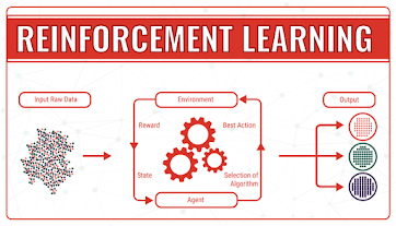

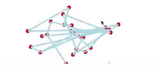
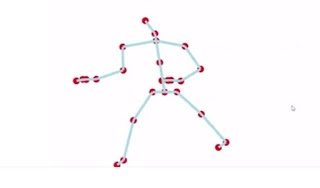
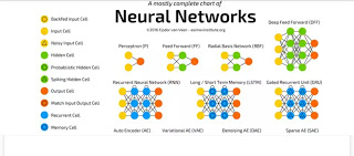


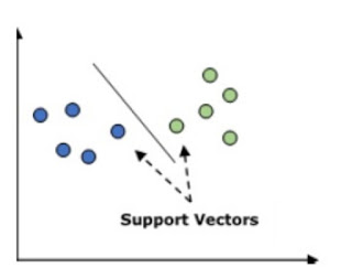
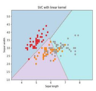
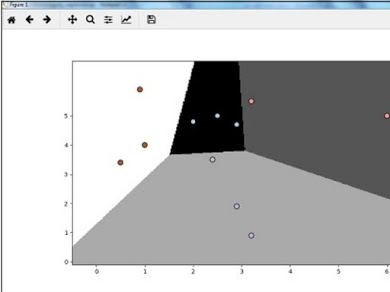
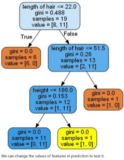
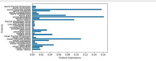
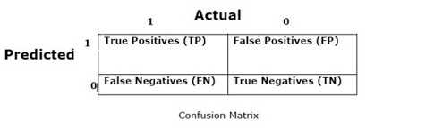
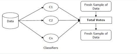
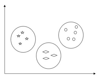
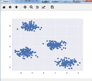
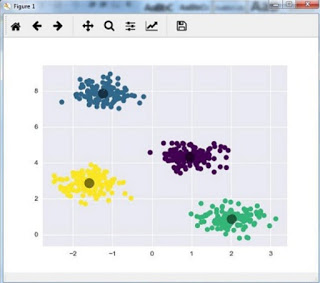
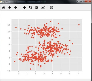
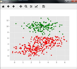
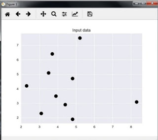
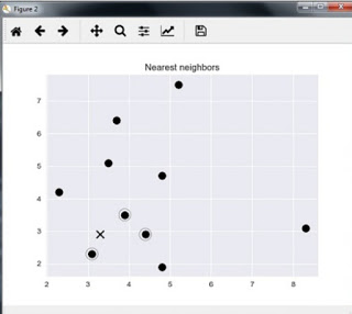

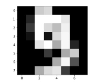
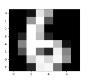
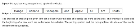
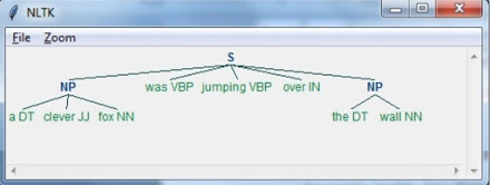
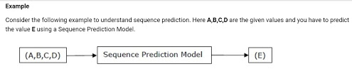
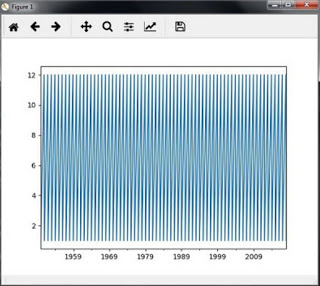
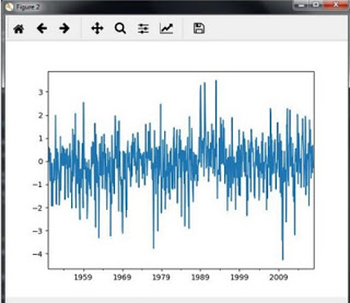
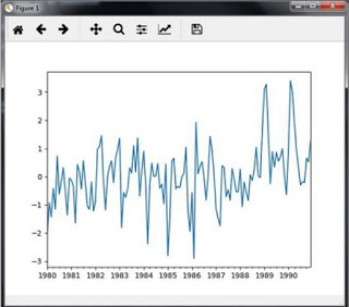
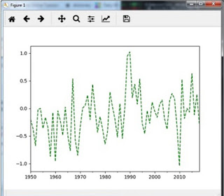
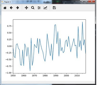
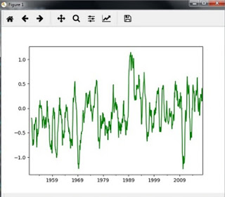
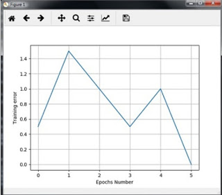
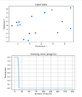
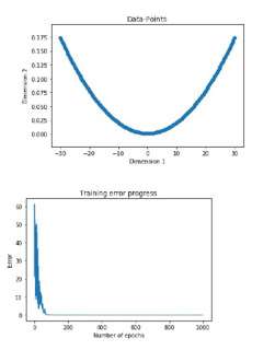
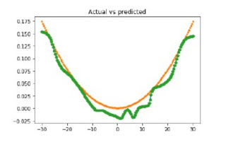
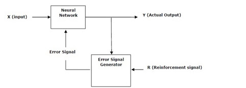
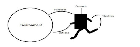
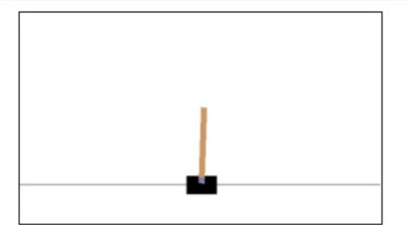
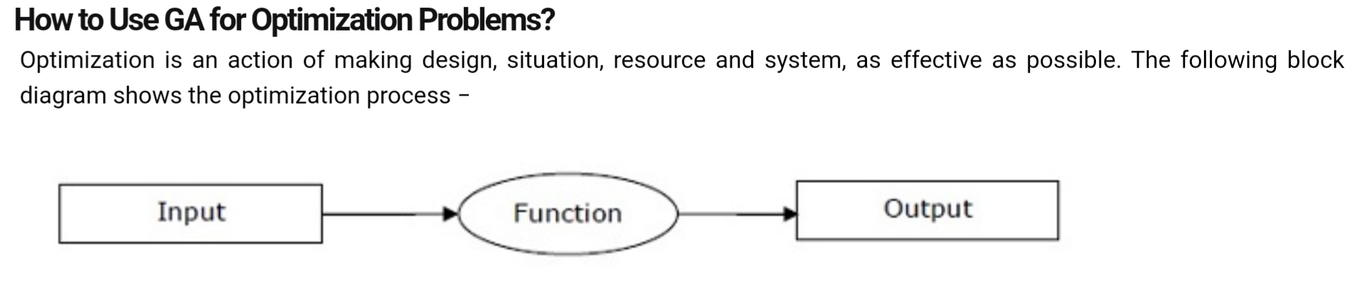
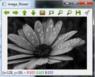


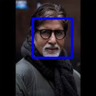

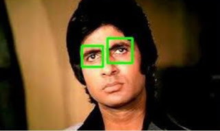


You must be logged in to post a comment.