Artificial Neural Network (ANN) it is an efficient computing system, whose central theme is borrowed from the analogy of biological neural networks. Neural networks are one type of model for machine learning. In the mid-1980s and early 1990s, much important architectural advancements were made in neural networks. In this chapter, you will learn more about Deep Learning, an approach of AI.

Deep learning emerged from a decade’s explosive computational growth as a serious contender in the field. Thus, deep learning is a particular kind of machine learning whose algorithms are inspired by the structure and function of human brain.

Machine Learning v/s Deep Learning

Deep learning is the most powerful machine learning technique these days. It is so powerful because they learn the best way to represent the problem while learning how to solve the problem. A comparison of Deep learning and Machine learning is given below −

Data Dependency

The first point of difference is based upon the performance of DL and ML when the scale of data increases. When the data is large, deep learning algorithms perform very well.

Machine Dependency

Deep learning algorithms need high-end machines to work perfectly. On the other hand, machine learning algorithms can work on low-end machines too.

Feature Extraction

Deep learning algorithms can extract high level features and try to learn from the same too. On the other hand, an expert is required to identify most of the features extracted by machine learning.

Time of Execution

Execution time depends upon the numerous parameters used in an algorithm. Deep learning has more parameters than machine learning algorithms. Hence, the execution time of DL algorithms, specially the training time, is much more than ML algorithms. But the testing time of DL algorithms is less than ML algorithms.

Approach to Problem Solving

Deep learning solves the problem end-to-end while machine learning uses the traditional way of solving the problem i.e. by breaking down it into parts.

Convolutional Neural Network (CNN)

Convolutional neural networks are the same as ordinary neural networks because they are also made up of neurons that have learnable weights and biases. Ordinary neural networks ignore the structure of input data and all the data is converted into 1-D array before feeding it into the network. This process suits the regular data, however if the data contains images, the process may be cumbersome.

CNN solves this problem easily. It takes the 2D structure of the images into account when they process them, which allows them to extract the properties specific to images. In this way, the main goal of CNNs is to go from the raw image data in the input layer to the correct class in the output layer. The only difference between an ordinary NNs and CNNs is in the treatment of input data and in the type of layers.

Architecture Overview of CNNs

Architecturally, the ordinary neural networks receive an input and transform it through a series of hidden layer. Every layer is connected to the other layer with the help of neurons. The main disadvantage of ordinary neural networks is that they do not scale well to full images.

The architecture of CNNs have neurons arranged in 3 dimensions called width, height and depth. Each neuron in the current layer is connected to a small patch of the output from the previous layer. It is similar to overlaying a 𝑵×𝑵filter on the input image. It uses M filters to be sure about getting all the details. These M filters are feature extractors which extract features like edges, corners, etc.

Layers used to construct CNNs

Following layers are used to construct CNNs −

·        Input Layer − It takes the raw image data as it is.

·        Convolutional Layer − This layer is the core building block of CNNs that does most of the computations. This layer computes the convolutions between the neurons and the various patches in the input.

·        Rectified Linear Unit Layer − It applies an activation function to the output of the previous layer. It adds non-linearity to the network so that it can generalize well to any type of function.

·        Pooling Layer − Pooling helps us to keep only the important parts as we progress in the network. Pooling layer operates independently on every depth slice of the input and resizes it spatially. It uses the MAX function.

·        Fully Connected layer/Output layer − This layer computes the output scores in the last layer. The resulting output is of the size 𝟏×𝟏×𝑳 , where L is the number training dataset classes.

Installing Useful Python Packages

You can use Keras, which is an high level neural networks API, written in Python and capable of running on top of TensorFlow, CNTK or Theno. It is compatible with Python 2.7-3.6. You can learn more about it from https://keras.io/.

Use the following commands to install keras −

pip install keras

On conda environment, you can use the following command −

conda install –c conda-forge keras

Building Linear Regressor using ANN

In this section, you will learn how to build a linear regressor using artificial neural networks. You can use KerasRegressor to achieve this. In this example, we are using the Boston house price dataset with 13 numerical for properties in Boston. The Python code for the same is shown here −

Import all the required packages as shown −

import numpy

import pandas

from keras.models import Sequential

from keras.layers import Dense

from keras.wrappers.scikit_learn import KerasRegressor

from sklearn.model_selection import cross_val_score

from sklearn.model_selection import KFold

Now, load our dataset which is saved in local directory.

dataframe = pandas.read_csv("/Usrrs/admin/data.csv", delim_whitespace = True, header = None)

dataset = dataframe.values

Now, divide the data into input and output variables i.e. X and Y −

X = dataset[:,0:13]

Y = dataset[:,13]

Since we use baseline neural networks, define the model −

def baseline_model():

Now, create the model as follows −

model_regressor = Sequential()

model_regressor.add(Dense(13, input_dim = 13, kernel_initializer = 'normal', 

   activation = 'relu'))

model_regressor.add(Dense(1, kernel_initializer = 'normal'))

Next, compile the model −

model_regressor.compile(loss='mean_squared_error', optimizer='adam')

return model_regressor

Now, fix the random seed for reproducibility as follows −

seed = 7

numpy.random.seed(seed)

The Keras wrapper object for use in scikit-learn as a regression estimator is called KerasRegressor. In this section, we shall evaluate this model with standardize data set.

estimator = KerasRegressor(build_fn = baseline_model, nb_epoch = 100, batch_size = 5, verbose = 0)

kfold = KFold(n_splits = 10, random_state = seed)

baseline_result = cross_val_score(estimator, X, Y, cv = kfold)

print("Baseline: %.2f (%.2f) MSE" % (Baseline_result.mean(),Baseline_result.std()))

The output of the code shown above would be the estimate of the model’s performance on the problem for unseen data. It will be the mean squared error, including the average and standard deviation across all 10 folds of the cross validation evaluation.

Image Classifier: An Application of Deep Learning

Convolutional Neural Networks (CNNs) solve an image classification problem, that is to which class the input image belongs to. You can use Keras deep learning library. Note that we are using the training and testing data set of images of cats and dogs from following link https://www.kaggle.com/c/dogs-vs-cats/data.

Import the important keras libraries and packages as shown −

The following package called sequential will initialize the neural networks as sequential network.

from keras.models import Sequential

The following package called Conv2D is used to perform the convolution operation, the first step of CNN.

from keras.layers import Conv2D

The following package called MaxPoling2D is used to perform the pooling operation, the second step of CNN.

from keras.layers import MaxPooling2D

The following package called Flatten is the process of converting all the resultant 2D arrays into a single long continuous linear vector.

from keras.layers import Flatten

The following package called Dense is used to perform the full connection of the neural network, the fourth step of CNN.

from keras.layers import Dense

Now, create an object of the sequential class.

S_classifier = Sequential()

Now, next step is coding the convolution part.

S_classifier.add(Conv2D(32, (3, 3), input_shape = (64, 64, 3), activation = 'relu'))

Here relu is the rectifier function.

Now, the next step of CNN is the pooling operation on the resultant feature maps after convolution part.

S-classifier.add(MaxPooling2D(pool_size = (2, 2)))

Now, convert all the pooled images into a continuous vector by using flattering −

S_classifier.add(Flatten())

Next, create a fully connected layer.

S_classifier.add(Dense(units = 128, activation = 'relu'))

Here, 128 is the number of hidden units. It is a common practice to define the number of hidden units as the power of 2.

Now, initialize the output layer as follows −

S_classifier.add(Dense(units = 1, activation = 'sigmoid'))

Now, compile the CNN, we have built −

S_classifier.compile(optimizer = 'adam', loss = 'binary_crossentropy', metrics = ['accuracy'])

Here optimizer parameter is to choose the stochastic gradient descent algorithm, loss parameter is to choose the loss function and metrics parameter is to choose the performance metric.

Now, perform image augmentations and then fit the images to the neural networks −

train_datagen = ImageDataGenerator(rescale = 1./255,shear_range = 0.2,

zoom_range = 0.2,

horizontal_flip = True)

test_datagen = ImageDataGenerator(rescale = 1./255)

training_set = 

   train_datagen.flow_from_directory(”/Users/admin/training_set”,target_size = 

      (64, 64),batch_size = 32,class_mode = 'binary')

test_set = 

   test_datagen.flow_from_directory('test_set',target_size = 

      (64, 64),batch_size = 32,class_mode = 'binary')

Now, fit the data to the model we have created −

classifier.fit_generator(training_set,steps_per_epoch = 8000,epochs = 

25,validation_data = test_set,validation_steps = 2000)

Here steps_per_epoch have the number of training images.

Now as the model has been trained, we can use it for prediction as follows −

from keras.preprocessing import image

test_image = image.load_img('dataset/single_prediction/cat_or_dog_1.jpg', 

target_size = (64, 64))

test_image = image.img_to_array(test_image)

test_image = np.expand_dims(test_image, axis = 0)

result = classifier.predict(test_image)

training_set.class_indices

if result[0][0] == 1:

prediction = 'dog'

else:

   prediction = 'cat'

                               “Deep learning Process”

A deep neural network provides state-of-the-art accuracy in many tasks, from object detection to speech recognition. They can learn automatically, without predefined knowledge explicitly coded by the programmers.

To grasp the idea of deep learning, imagine a family, with an infant and parents. The toddler points objects with his little finger and always says the word ‘cat.’ As its parents are concerned about his education, they keep telling him ‘Yes, that is a cat’ or ‘No, that is not a cat.’ The infant persists in pointing objects but becomes more accurate with ‘cats.’ The little kid, deep down, does not know why he can say it is a cat or not. He has just learned how to hierarchies complex features coming up with a cat by looking at the pet overall and continue to focus on details such as the tails or the nose before to make up his mind.

A neural network works quite the same. Each layer represents a deeper level of knowledge, i.e., the hierarchy of knowledge. A neural network with four layers will learn more complex feature than with that with two layers.

The learning occurs in two phases.

• The first phase consists of applying a nonlinear transformation of the input and create a statistical model as output.
• The second phase aims at improving the model with a mathematical method known as derivative.

The neural network repeats these two phases hundreds to thousands of time until it has reached a tolerable level of accuracy. The repeat of this two-phase is called an iteration.

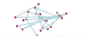
To give an example, take a look at the motion below, the model is trying to learn how to dance. After 10 minutes of training, the model does not know how to dance, and it looks like a scribble.

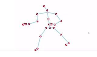
After 48 hours of learning, the computer masters the art of dancing.

Classification of Neural Networks

Shallow neural network: The Shallow neural network has only one hidden layer between the input and output.

Deep neural network: Deep neural networks have more than one layer. For instance, Google LeNet model for image recognition counts 22 layers.

Nowadays, deep learning is used in many ways like a driverless car, mobile phone, Google Search Engine, Fraud detection, TV, and so on.

Types of Deep Learning Networks

Feed-forward neural networks

The simplest type of artificial neural network. With this type of architecture, information flows in only one direction, forward. It means, the information’s flows starts at the input layer, goes to the “hidden” layers, and end at the output layer. The network does not have a loop. Information stops at the output layers.

Recurrent neural networks (RNNs)

RNN is a multi-layered neural network that can store information in context nodes, allowing it to learn data sequences and output a number or another sequence. In simple words it an Artificial neural networks whose connections between neurons include loops. RNNs are well suited for processing sequences of inputs.

Example, if the task is to predict the next word in the sentence “Do you want a…………?

• The RNN neurons will receive a signal that point to the start of the sentence.
• The network receives the word “Do” as an input and produces a vector of the number. This vector is fed back to the neuron to provide a memory to the network. This stage helps the network to remember it received “Do” and it received it in the first position.
• The network will similarly proceed to the next words. It takes the word “you” and “want.” The state of the neurons is updated upon receiving each word.
• The final stage occurs after receiving the word “a.” The neural network will provide a probability for each English word that can be used to complete the sentence. A well-trained RNN probably assigns a high probability to “café,” “drink,” “burger,” etc.

Common uses of RNN

• Help securities traders to generate analytic reports
• Detect abnormalities in the contract of financial statement
• Detect fraudulent credit-card transaction
• Provide a caption for images
• Power chatbots
• The standard uses of RNN occur when the practitioners are working with time-series data or sequences (e.g., audio recordings or text).  

       “Composing Jazz Music with Deep Learning”

Deep Learning is on the rise, extending its application in every field, ranging from computer vision to natural language processing, healthcare, speech recognition, generating art, addition of sound to silent movies, machine translation, advertising, self-driving cars, etc. In this blog, we will extend the power of deep learning to the domain of music production. We will talk about how we can use deep learning to generate new musical beats.

The current technological advancements have transformed the way we produce music, listen, and work with music. With the advent of deep learning, it has now become possible to generate music without the need for working with instruments artists may not have had access to or the skills to use previously. This offers artists more creative freedom and ability to explore different domains of music.

Recurrent Neural Networks

Since music is a sequence of notes and chords, it doesn’t have a fixed dimensionality. Traditional deep neural network techniques cannot be applied to generate music as they assume the inputs and targets/outputs to have fixed dimensionality and outputs to be independent of each other. It is therefore clear that a domain-independent method that learns to map sequences to sequences would be useful.

Recurrent neural networks (RNNs) are a class of artificial neural networks that make use of sequential information present in the data.

A recurrent neural network has looped, or recurrent, connections which allow the network to hold information across inputs. These connections can be thought of as memory cells. In other words, RNNs can make use of information learned in the previous time step. As seen in Fig. 1, the output of the previous hidden/activation layer is fed into the next hidden layer. Such an architecture is efficient in learning sequence-based data.

In this blog, we will be using the Long Short-Term Memory (LSTM) architecture. LSTM is a type of recurrent neural network (proposed by Hochreiter and Schmidhuber, 1997) that can remember a piece of information and keep it saved for many timesteps.

Dataset

Our dataset includes piano tunes stored in the MIDI format. MIDI (Musical Instrument Digital Interface) is a protocol which allows electronic instruments and other digital musical tools to communicate with each other. Since a MIDI file only represents player information, i.e., a series of messages like ‘note on’, ‘note off, it is more compact, easy to modify, and can be adapted to any instrument.

Before we move forward, let us understand some music related terminologies:

·        Note: A note is either a single sound or its representation in notation. Each note consist of pitch, octave, and an offset.

·        Pitch: Pitch refers to the frequency of the sound.

·        Octave: An octave is the interval between one musical pitch and another with half or double its frequency.

·        Offset: Refers to the location of the note.

·        Chord: Playing multiple notes at the same time constitutes a chord.

Machine Learning vs Deep Learning: What’s the Difference?

AI has three different levels:

1. Narrow AI: A artificial intelligence is said to be narrow when the machine can perform a specific task better than a human. The current research of AI is here now
2. General AI: An artificial intelligence reaches the general state when it can perform any intellectual task with the same accuracy level as a human would
3. Active AI: An AI is active when it can beat humans in many tasks

What is ML?

Machine learning is the best tool so far to analyze, understand and identify a pattern in the data. One of the main ideas behind machine learning is that the computer can be trained to automate tasks that would be exhaustive or impossible for a human being. The clear breach from the traditional analysis is that machine learning can take decisions with minimal human intervention.

Machine learning uses data to feed an algorithm that can understand the relationship between the input and the output. When the machine finished learning, it can predict the value or the class of new data point.

What is Deep Learning?

Deep learning is a computer software that mimics the network of neurons in a brain. It is a subset of machine learning and is called deep learning because it makes use of deep neural networks. The machine uses different layers to learn from the data. The depth of the model is represented by the number of layers in the model. Deep learning is the new state of the art in term of AI. In deep learning, the learning phase is done through a neural network. A neural network is an architecture where the layers are stacked on top of each other

Machine Learning Process

Imagine you are meant to build a program that recognizes objects. To train the model, you will use a classifier. A classifier uses the features of an object to try identifying the class it belongs to.

In the example, the classifier will be trained to detect if the image is a:

• Bicycle
• Boat
• Car
• Plane

The four objects above are the class the classifier has to recognize. To construct a classifier, you need to have some data as input and assigns a label to it. The algorithm will take these data, find a pattern and then classify it in the corresponding class.

This task is called supervised learning. In supervised learning, the training data you feed to the algorithm includes a label.

Training an algorithm requires to follow a few standard steps:

• Collect the data
• Train the classifier
• Make predictions

The first step is necessary, choosing the right data will make the algorithm success or a failure. The data you choose to train the model is called a feature. In the object example, the features are the pixels of the images.

Each image is a row in the data while each pixel is a column. If your image is a 28×28 size, the dataset contains 784 columns (28×28). In the picture below, each picture has been transformed into a feature vector. The label tells the computer what object is in the image.

The objective is to use these training data to classify the type of object. The first step consists of creating the feature columns. Then, the second step involves choosing an algorithm to train the model. When the training is done, the model will predict what picture corresponds to what object.

After that, it is easy to use the model to predict new images. For each new image feeds into the model, the machine will predict the class it belongs to. For example, an entirely new image without a label is going through the model. For a human being, it is trivial to visualize the image as a car. The machine uses its previous knowledge to predict as well the image is a car.

Deep Learning Process

In deep learning, the learning phase is done through a neural network. A neural network is an architecture where the layers are stacked on top of each other.

Consider the same image example above. The training set would be fed to a neural network

Each input goes into a neuron and is multiplied by a weight. The result of the multiplication flows to the next layer and become the input. This process is repeated for each layer of the network. The final layer is named the output layer; it provides an actual value for the regression task and a probability of each class for the classification task. The neural network uses a mathematical algorithm to update the weights of all the neurons. The neural network is fully trained when the value of the weights gives an output close to the reality. For instance, a well-trained neural network can recognize the object on a picture with higher accuracy than the traditional neural net.

Automate Feature Extraction using DL

A dataset can contain a dozen to hundreds of features. The system will learn from the relevance of these features. However, not all features are meaningful for the algorithm. A crucial part of machine learning is to find a relevant set of features to make the system learns something.

One way to perform this part in machine learning is to use feature extraction. Feature extraction combines existing features to create a more relevant set of features. It can be done with PCA, T-SNE or any other dimensionality reduction algorithms.

For example, an image processing, the practitioner needs to extract the feature manually in the image like the eyes, the nose, lips and so on. Those extracted features are feed to the classification model.

Deep learning solves this issue, especially for a convolutional neural network. The first layer of a neural network will learn small details from the picture; the next layers will combine the previous knowledge to make more complex information. In the convolutional neural network, the feature extraction is done with the use of the filter. The network applies a filter to the picture to see if there is a match, i.e., the shape of the feature is identical to a part of the image. If there is a match, the network will use this filter. The process of feature extraction is therefore done automatically.

Difference between Machine Learning and Deep Learning

	Machine Learning	Deep Learning
Data Dependencies	Excellent performances on a small/medium dataset	Excellent performance on a big dataset
Hardware dependencies	Work on a low-end machine.	Requires powerful machine, preferably with GPU: DL performs a significant amount of matrix multiplication
Feature engineering	Need to understand the features that represent the data	No need to understand the best feature that represents the data
Execution time	From few minutes to hours	Up to weeks. Neural Network needs to compute a significant number of weights
Interpretability	Some algorithms are easy to interpret (logistic, decision tree), some are almost impossible (SVM, XGBoost)	Difficult to impossible

When to use ML or DL?

In the table below, we summarize the difference between machine learning and deep learning.

	Machine learning	Deep learning
Training dataset	Small	Large
Choose features	Yes	No
Number of algorithms	Many	Few
Training time	Short	Long

With machine learning, you need fewer data to train the algorithm than deep learning. Deep learning requires an extensive and diverse set of data to identify the underlying structure. Besides, machine learning provides a faster-trained model. Most advanced deep learning architecture can take days to a week to train. 

The advantage of deep learning over machine learning is it is highly accurate. You do not need to understand what features are the best representation of the data; the neural network learned how to select critical features. In machine learning, you need to choose for yourself what features to include in the model.